FLEXIBLE FRAMEWORK FOR MODELING WATER
CONVEYANCE NETWORKS
Jo˜ao Miguel Lemos Chasqueira Nabais
IDMEC, Department of Systems and Informatics, Escola Superior de Tecnologia de Set´ubal
Campus do IPS, Estefanilha 2910-761 Set´ubal, Portugal
Jos´e Duarte
Departamento de Inform´atica, Universidade de
´
Evora, Rua Rom˜ao Ramalho 59, 7000-671
´
Evora, Portugal
Miguel Ayala Botto
IDMEC, Instituto Superior T´ecnico, Technical University of Lisbon, Av. Rovisco Pais, 1049-001 Lisboa, Portugal
Manuel Rijo
NuHCC - Hydraulics and Canal Control Center, Universidade de
´
Evora
P´olo da Mitra Apartado 94, 7002–554
´
Evora, Portugal
Keywords:
Water Delivery Canals, Modeling, Network Transportation Systems, Leak Detection, Fault Tolerant Control.
Abstract:
A flexible framework for modeling different water conveyance networks is presented. The network is modeled
using a linear canal pool model based on the Saint-Venant equations to describe transportation phenomenon
occurring in open channels. This model is used as a link to connect different nodes defined by gates or
reservoirs. The linear pool model has interesting features namely the pool axis monitoring, the inflow along
the pool axis and the ability to consider different boundary conditions. Based on these characteristics canal
pool observers for leak detection and localization can be developed. It is shown that based on a finite difference
scheme a good performance is obtained for low space resolution. The modeling framework is validated with
experimental data from a real canal property of the
´
Evora University. This is a challenging configuration due
to its strong canal pool coupling.
1 INTRODUCTION
Water is vital for mankind way of life. It is used for
multiple purposes, essential for agricultural and in-
dustry, domestic use and even for recreation. Unfor-
tunately, water is becoming a rare resource so contri-
butions to increase water use efficiency are welcome.
As the water source is not always close to the end
users there exists the need to create efficient system,
or network, to execute the water conveyance. The
water transportation problem is not exclusively ded-
icated to delivery water to users. Water has also to
be transported to safety locations rendering the man-
agement of water systems a complex task. Complex
water transportation systems span from small-scale to
large distributed systems, as is the case of large rivers
that often crosses different countries. Water trans-
portation systems may be divided into the following
categories (Negenborn et al., 2009),
Irrigations Canals: are responsible for transporting
water often from a long distance source, to the
users. The objective is to deliver the specified
amount of water that is normally accomplished by
controlling the water depth at the extraction local-
ization;
Sewers Networks: these systems are responsible to
transport the waste water (from houses or due to
rain) to treatment plants. The objective is to avoid
water contamination and also execute flood con-
trol;
Large Multi-purpose Reservoirs: the course of
natural rivers are controlled by large dams in
order to create a large water storage capacity
that can be used for different objectives as power
142
Miguel Lemos Chasqueira Nabais J., Duarte J., Ayala Botto M. and Rijo M..
FLEXIBLE FRAMEWORK FOR MODELING WATER CONVEYANCE NETWORKS.
DOI: 10.5220/0003598101420147
In Proceedings of 1st International Conference on Simulation and Modeling Methodologies, Technologies and Applications (SIMULTECH-2011), pages
142-147
ISBN: 978-989-8425-78-2
Copyright
c
 2011 SCITEPRESS (Science and Technology Publications, Lda.)

production, irrigation and flood control.
Open-channels models are mainly divided into
physical principle models and data driven mod-
els (Zhuan and Xia, 2007). Physical principle mod-
els (Litrico and Fromion, 2009) are based on the pro-
cess knowledge. In particular, for canal systems they
are based on the Saint-Venant equations and on the
geometrical and hydraulic system description. Natu-
rally, the model performance is dependent on the sys-
tem parameters accuracy, for high uncertainty param-
eter the performance decreases. They are also use-
ful as they can give some physical insight in the con-
trol engineering design phase. Data driven models are
based on identification tools leading to grey or black
box models (Weyer, 2001). These methods require
the physical existence of the canal but can produce a
model with a high level of accuracy.
In this paper, a flexible framework for modeling
water transportation networks is presented. The canal
pool dynamics is the most relevant component as it
is responsible for the transportation phenomena; in
particular it is important to have a model capable of
capturing the backwater, or by other words, the water
profile along the pool axis, the wave translation and
attenuation as well as the flow acceleration . Special
features made available in this framework are due to
the pool model (Nabais and Botto, 2011). In particu-
lar, with this canal pool model it is possible to,
• monitor the pool axis in water depth and discharge
as the white box state space vector is composed by
this information. In the presence of few sensors,
the model can be used as an observer to predict the
water depth along the pool axis and verify for ex-
ample the danger of occurring overtopping. Using
this ability the purposed model can also be used
for the development of pool observers;
• execute outflows or inflows along the pool axis.
With this feature it will be possible to proceed
with the leak identification and localization on ir-
rigation networks while for drainage systems it
will be possible to account for additional water
inflows in the case of torrential rains, for instance;
• choose the boundary condition as discharge im-
posed by an hydraulic structure, or water depth
imposed by a reservoir, and model multipurpose
reservoir systems using the pool model to connect
different reservoirs;
• as the linear pool model is given as a state space
representation, the dynamics are solved through
matrices multiplications, with a low computa-
tional cost. This is of capital importance for large
scale systems as computation effort may impose a
limit to the largest tractable system dimension;
• extracting linear models for the local dynamics
pool plus gate is straightforward, the boundary
condition is replaced by the hydraulic linearized
equation.
The paper has the following structure. Section 2
presents the experimental water delivery canal hold
by the NuHCC – Hydraulics and Canal Control Cen-
ter from the
´
Evora University in Portugal. The wa-
ter transportation system typical components – canal
pools, discharge and water depth control structures
and storage elements – are presented in section 3. The
canal pool dynamics is solved by linearization ans dis-
cretization of the Saint-Venant equations, the reser-
voirs are modeled as an integrator element and the
gates are described by static relations. In section 4 a
brief description of the developed MatLab–Simulink
Toolbox–Library is given. In section 5 the purposed
modeling framework is validated for the experimen-
tal canal. Here it is shown the reliability, accuracy
and flexibility of the proposed hydraulic model for a
wide range of inputs. Finally, in section 6 some con-
clusions are drawn.
2 EXPERIMENTAL CANAL
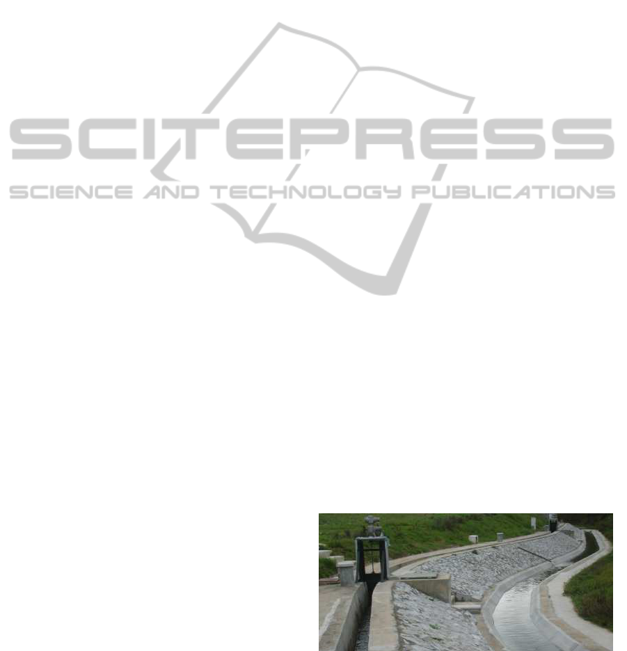
The experimental automatic canal, property of
NuHCC is located in Mitra near
´
Evora in Portu-
gal. The canal is built with trapezoidal section (with
0.15m bottom width and 1 : 0.15 side slope), a maxi-
mum height of 0.9m, 145m length and an average lon-
gitudinal bottom slope about 0.0015. The canal works
in closed loop to avoid water spillage, and the return
flow to the reservoir is secured by a second canal (a
traditional local upstream controlled canal Figure1).
The water is pumped from the lower reservoir to the
higher reservoir by two pumps. The canal inflow is
controlled by an electrical MONOVAR valve located
downstream the higher reservoir. The facility was de-
signed for a maximum discharge of 0.090m
3
/s.
Figure 1: NuHCC canal property of
´
Evora University.
In its basic configuration, the automatic canal is
divided into four pools by three undershot gates and
FLEXIBLE FRAMEWORK FOR MODELING WATER CONVEYANCE NETWORKS
143

an overshot gate (vertical), this one located at the
downstream canal section. Upstream each gate there
exist an offtake, equipped with flow meter and an
electrical butterfly, to allow water user extraction, and
discharges into the return traditional canal. Float and
counter-weight level sensors are distributed along the
canal axis, three in each pool, allowing for water
depth canal monitoring.
The facility has a 6 PLC network: five local,
assigned to each gate and reservoirs, connected by
a MODBUS network to the central master PLC.
The master PLC communicates to the SCADA com-
puter by a serial port RS232 interface. Recently,
a SCADA-Controller Interface application has been
developed (Duarte et al., 2011) allowing interaction
with the facility through different environments as
MatLab, C/C++ and GNU Prolog.
3 WATER TRANSPORTATION
NETWORKS
Water conveyance networks are complex systems
usually space distributed with a large dimension. Like
other network systems they are composed by links
and nodes. The link between nodes is accomplish
by the water transportation element – the pool. The
nodes establish the separation of different links and
are represented by reservoir, gates or a combination
of both.
3.1 Pool Dynamics
The flow dynamics in open channels is well described
by the Saint-Venant equations (Akan, 2006), nonlin-
ear partial differential equations of hyperbolic type
capable of describing the transport phenomenon,
∂Q(x,t)
∂x
+ T(x,t)
∂Y(x,t)
∂t
= 0 (1)
∂Q(x,t)
∂t
+
∂
∂x

Q
2
(x,t)
A(x,t)

+ . . .
. . . + g· A(x,t) · (S
f
(x,t) − S
0
(x)) = 0 (2)
where, A(x,t) is the wetted cross section, Q(x, t) is
the water discharge, Y(x,t) is the water depth, T(x, t)
is the wetted cross section top width, S
f
(x,t) is the
friction slope, S
0
(x) is the bed slope, x and t are the
independent variables. One approach to this com-
plex problem is to linearize (1) (2) around a nonuni-
form steady configuration defined by (Q
0
,Y(L, 0)).
To help future analysis is useful to consider the area
deviation as a(x,t) = T
0
(x)y(x,t) and the state vector
χ(x,t) =

q(x,t) a(x, t)

T
. The linearized Saint-
Venant equations can be expressed in state space form
as follows,
ˆ
A
∂
∂t
χ(x,t) +
ˆ
B(x)
∂
∂x
χ(x,t) +
ˆ
C(x)χ(x, t) = 0 (3)
where matrices
ˆ
A,
ˆ
B(x) and
ˆ
C(x) are defined
in (Litrico and Fromion, 2009). Numerical methods
are known to introduce nonphysical behavior that is
similar to the process physics and is not clear how to
eliminate it (Szymkiewicz, 2010). The Preissmman
scheme is the numerical method used to discretize the
linearized Saint-Venant equations. The parameters φ
and θ are weighting parameters for space and time
respectively and vary between 0 and 1. The index i
stands for section while index k stands for time itera-
tion.
The flow dynamics between two adjacent sections
is described by (Nabais and Botto, 2011),
¯
Ax(k+ 1) +
¯
Bx(k) =
¯
B
w
w(k+ 1, k) (4)
where x(k) =

q
k
i
a
k
i
q
k
i+1
a
k
i+1

T
is the sec-
tion i state space vector and w(k + 1, k) =
h
q
k
of f
q
k+1
of f
i
T
represents the discharge perturba-
tion between sections i and i + 1 where q
of f
means
the lateral outflow. The pool flow dynamic model is
obtained interconnecting N section models (4) lead-
ing to 2N equations. The state space vector,
X(k) =

q
1
(k) a
1
(k) q
2
(k) a
2
(k) . . .
. . . q
n
(k) a
n
(k) q
n+1
(k) a
n+1
(k)

(5)
has dimension 2(N + 1). To complete the model it is
necessary to add boundary conditions. As the flow
is considered subcritical one boundary condition for
each end is introduced.
3.1.1 Boundary Equations
In the case of water discharge, when the pool is con-
nected to an hydraulic structure as a gate or a pump,
the boundary condition can be written as u = q
k+1
which means the model command signal is the next
discharge value. In state space this is equivalent to,

1 0


q
k+1
i
a
k+1
i

+

0 0


q
k
i
a
k
i

= u (6)
A similar approach is done for the water depth
boundary condition, when the pool is connected to an
hydraulic structure or reservoir, written as u = y
k+1
so the model command signal is the next water depth
value. In state space form this is equivalent to,

0 1


q
k+1
i
a
k+1
i

+

0 0


q
k
i
a
k
i

= T
i
u (7)
SIMULTECH 2011 - 1st International Conference on Simulation and Modeling Methodologies, Technologies and
Applications
144

3.1.2 Linear Pool Model
After the boundary addition, the pool linear model is
given as,
X(k+ 1) = AX(k) + BU(k) + B
w
W(k, k − 1)
Y(k) = CX(k) + D
v
V(k) (8)
where X(k) is the state space vector, Y(k) is the out-
put, U(k) is the model input, W(k) is the state space
perturbation in discharge and V(k) is the output per-
turbation.
3.1.3 Model Analysis
The model tunable parameters guidelines are pre-
sented bellow:
• the number of sections considered, N, should be a
compromise between computation effort and ac-
curacy, and fixes the space step;
• the sample time should be tuned to maintain the
Courant number C
r
= α
∆t
δx
(where α is the down-
stream wave velocity, ∆t is the sample time and ∆x
is the space step) close to unity. This is the same
to say that the space and time resolution should be
equivalent;
• for the discretization parameters, the φ = 0.5 is
imposed to work in the centered configuration that
is known to be unconditionally stable for θ ≥ 0.5.
In particular, θ should be chosen θ > 0.5 to in-
troduce numerical diffusion to eliminate the nu-
merical oscillations introduced by the numerical
method.
The model also allows for some hydraulic param-
eters calibration, namely the Manning hydraulic coef-
ficient and the gates discharge coefficient.
3.2 Hydraulic Structures
The flow in open-channel networks is usually con-
trolled by hydraulic structures. For the irrigation ap-
plication, these structures are usually gates. These
gates can be classified as overshot gates, with the flow
over the gate, or undershoot gates, with the flow under
the gate. Only consideringfree flow conditions for the
first type and submerged flow conditions for the last
one (the usually conditions in this type of canals) the
gate equations are respectively (Laycock, 2007),
Q
g
= cd · L
g
·
p
2g(Y
u
−Y
g
)
3
2
(9)
Q
g
= cd · A
g
·
p
2g
p
Y
u
−Y
d
(10)
where cd is the gate discharge coefficient, A
g
is the
gate submerged orifice, L
g
is the gate top width and
Y
g
is the gate height.
3.3 Reservoirs
The reservoirs are the nodes in a water conveyance
network. They exhibit an integral behavior and the
reservoir water depth can be modeled by the follow-
ing difference equation (Moudgalya, 2007),
h(k+ 1) = h(k) +
T
s
A
s
q
i
(k) −
T
s
A
s
q
o
(k) (11)
where T
s
means the sample time, A
s
the superficial
area, q
i
(k) the inflow and q
o
(k) the outflow.
4 MATLAB–SIMULINK
TOOLBOX–LIBRARY
A MatLab
c

–Simulink
c

Toolbox–Library has been
developed. It is a two stage product. In MatLab
c

the pool models are created and in Simulink
c

the ele-
mentary components are available as blocks for creat-
ing canal configurations. The toolbox was developed
with special attention to create a flexible and modu-
lar product. The elementary blocks (pools, gates and
reservoirs) are available in the library and by inter-
connecting them it is possible to create different canal
configurations. Using different canal configurations,
a water conveyance network can be created.
The Library is divided into five categories:
Pool Models: beyond the linear pool model pre-
sented also a simplified infinite dimension pool
model named Integrator Delay Zero (Litrico and
Fromion, 2004) (IDZ) is available;
Standard Canal Configurations: some typical
canal configurations are made available: for one,
two and four pools configurations;
Gates: the overshot and undershot gate equations are
implemented for the sections considered above. It
makes use of the geometry component for com-
puting the gate discharge. Expansion to other
geometries is made through a simple parameter
change – in the cross section or top width;
Hardware: in this section some hardware static rela-
tions are available. The gate dynamics is defined
through both saturation in amplitude and varia-
tion. The valves controlling the canal discharges,
canal intake and offtakes, are sufficiently well ap-
proximated by a first order system with a time de-
lay;
Geometry: computes the hydraulic cross section pa-
rameters for different geometries, to know: area,
wetted perimeter, hydraulic radius, top width and
hydraulic depth.
FLEXIBLE FRAMEWORK FOR MODELING WATER CONVEYANCE NETWORKS
145

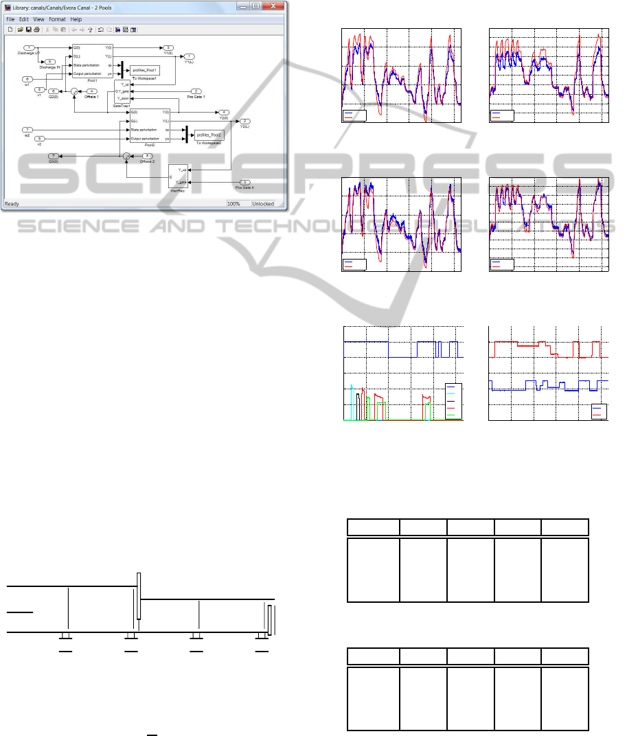
In Figure 2 is represented the two pool canal configu-
ration. As this is a MatLab
c

–Simulink
c

Toolbox–
Library all canals composed by two pools use the
same Simulink
c

model, they only differ on the ge-
ometric characteristics in pools and gates leading to
distinct dynamics calculated by the MatLab
c

Tool-
box.
Figure 2: General view for a two pool configuration canal.
5 EXPERIMENTAL RESULTS
A simulator for the used experimental canal was built
using the toolbox presented. For model validation, the
canal was considered divided into two pools, which is
equivalent to say that gates 1 and 3 are totally opened.
In this configuration it is possible to proceed with wa-
ter extraction along the canal pools axis which is rel-
evant to validate the model.
The interaction with the canal is done through 7
inputs namely Figure 3, u
1
the upstream inflow, u
2
gate elevation for upstream pool, u
3
gate elevation
for downstream pool, d
1
offtake located upstream the
gate u
2
, d
2
offtake located upstream the gate u
3
, w
1
outflow at upstream pool center, w
2
outflow at down-
stream pool center. The model outputs was chosen as
the center (y
1
, y
3
) and downstream water depth (y
2
,
y
4
) in each pool.
4
) in each pool.
-
1
6
1
@
@
1
6
2
@
@
1
6
2
6
3
@
@
2
6
4
Z
Z
@
@
2
6
3
Figure 3: Schematics of the complete facility.
Figure 3: Schematics of the complete facility.
The linear pool model has the following numerical
parameters, N = 10, ∆x =
L
i
10
, ∆t = 3.3s, θ = 0.6 and
φ = 0.5. Several tests were made for this canal con-
figuration; Test A: sequence with u
1
, u
2
and u
4
, about
2700s; Test B: step sequence in w
1
and w
3
, about
3240s; Test C: short sequence with all inputs, about
6000s; Test D: long sequence with all inputs manip-
ulated Figure 4, about 26000s. The model perfor-
mance is quantified through the Variance Accounted
For (VAF) and Root Square Error (RSE), Table 1 – 2.
0 0.5 1 1.5 2 2.5
x 10
4
0.5
0.55
0.6
0.65
0.7
0.75
time [s]
water depth [m]
Canal
Model
(a) Downstream water level for
pool 1 y
2
.
0 0.5 1 1.5 2 2.5
x 10
4
0.5
0.52
0.54
0.56
0.58
0.6
0.62
0.64
0.66
0.68
0.7
time [s]
water depth [m]
Canal
Model
(b) Downstream water level for
pool 2, y
4
.
0 0.5 1 1.5 2 2.5
x 10
4
0.45
0.5
0.55
0.6
0.65
0.7
time [s]
water depth [m]
Canal
Model
(c) Center water depth at up-
stream pool y
1
.
0 0.5 1 1.5 2 2.5
x 10
4
0.46
0.48
0.5
0.52
0.54
0.56
0.58
0.6
0.62
0.64
0.66
time [s]
water depth [m]
Canal
Model
(d) Center water depth at down-
stream pool y
3
.
0 0.5 1 1.5 2 2.5
x 10
4
0
0.01
0.02
0.03
0.04
0.05
0.06
time [s]
discharge [m
3
/s]
u
1
d
1
d
2
w
1
w
2
(e) Input discharges.
0 0.5 1 1.5 2 2.5
x 10
4
0
0.1
0.2
0.3
0.4
0.5
time [s]
elevation [m]
u
2
u
3
(f) Gates elevation.
Figure 4: White box model validation for Test D.
Table 1: VAF criteria for the considered water depths.
VAF y
1
y
2
y
3
y
4
Test A 86.61 75.19 97.52 93.68
Test B 92.83 89.86 83.26 73.14
Test C 95.45 89.30 98.11 87.35
Test D 97.29 91.41 97.22 88.71
Table 2: RSE criteria for the considered water depths.
RSE y
1
y
2
y
3
y
4
Test A 0.018 0.017 0.005 0.008
Test B 0.009 0.011 0.005 0.006
Test C 0.008 0.013 0.005 0.012
Test D 0.013 0.015 0.007 0.015
SIMULTECH 2011 - 1st International Conference on Simulation and Modeling Methodologies, Technologies and
Applications
146

The best water depth VAF corresponds to cen-
ter pool localizations. Upstream each gate the ob-
served VAF decrease is explained for the gate dynam-
ics accuracy, in particular at the downstream overshot
gate. The water depth upstream the overshot gate is
strongly influenced by the existing leak. Naturally,
the leak intensity is a function of the water depth and
this is the reason why the absolute error increases for
higher water depths Figure 4(b). As the pools are in
a backwater mode, the water depth error is attenuated
when moving upstream as the water depth is tending
to the normal depth.
Finite difference methods usually require a high
space resolution to guarantee a good performance.
For the model proposed this is equivalent to grow the
N + 1 number of sections considered for a pool. The
important issue is to have some information about a
good tradeoff between computational cost and model
accuracy. To this end the simulator was tested consid-
ering different number of sections for the pool, in par-
ticular N =

10 20 30

. The models compari-
son performance is done for 1800s test duration, Ta-
ble 3. As expected, the computational time increases
with the space resolution but the model performance
is similar. A good performance is achieved for a low
space resolution which means that the pool model di-
mension stays tractable.
Table 3: Computational cost for a 1800s test duration.
MAE N = 10 N = 20 N = 30
Time [s] 2.5 14 41
VAF
y
1
94.67 92.62 91.77
VAF
y
2
94.23 94.18 94.15
VAF
y
3
66.29 62.65 60.75
VAF
y
4
71.59 71.57 71.55
6 CONCLUSIONS
A flexible framework toolbox for constructing wa-
ter conveyance networks has been presented and val-
idated on an experimental automatic canal. The aug-
mented model representation for the transportation el-
ement although based on a finite difference scheme
offers a good performance for low space resolution.
The purposed model opens new research directions.
The ability to account for water extraction along the
pool can support the development of leak detection
and localization algorithms. The pool monitoring ca-
pacity allows also for observer design.
ACKNOWLEDGEMENTS
This work was supported by the Portuguese Govern-
ment, through Fundac¸˜ao para a Ciˆencia e a Tecnolo-
gia, under the project PTDC/EEACRO/102102/2008
- AQUANET, IDMEC.
REFERENCES
Akan, A. O. (2006). Open Channel Hydraulics. Elsevier.
Duarte, J., Rato, L., Shirley, P., and Rijo, M. (2011). Multi-
platform controller interface for scada application. In
IFAC World Congress (Accepted in), Milan, Italy.
Laycock, A. (2007). Irrigation Systems: design, planning
and construction. CAB International.
Litrico, X. and Fromion, V. (2004). Simplified modeling
of irrigation canals for controller design. Journal of
Irrigation and Drainage Engineering, 130:373–383.
Litrico, X. and Fromion, V. (2009). Modeling and Control
of Hydrosystems. Springer-Verlag.
Moudgalya, K. (2007). Digital Control. Wiley.
Nabais, J. and Botto, M. A. (2011). Linear model for canal
pools. In 8th Internation Conference on Informatics
in Control, Automation and Robotics (Accepted in),
Noordwijkerhout, The Netherlands.
Negenborn, R., van Overloop, P.-J., Keviczky, T., and
de Schutter, B. (2009). Distributed model predictive
control of irrigation canals. Networks and Heteroge-
neous Media, 4(2):359–380.
Szymkiewicz, R. (2010). Numerical Modeling in Open
Channel. Springer-Verlag.
Weyer, E. (2001). System identification of an open water
channel. Control Engineering Practice, 9:1289–1299.
Zhuan, X. and Xia, X. (2007). Models and control method-
ologies in open water flow dynamics: A survey. In
8th IEEE Africon Conference, pages 1–7, Windhoek,
Namibia.
FLEXIBLE FRAMEWORK FOR MODELING WATER CONVEYANCE NETWORKS
147