
DEDICATED VS. ON-DEMAND INFRASTRUCTURE COSTS
IN COMMUNICATIONS-INTENSIVE APPLICATIONS
Oleksiy Mazhelis, Pasi Tyrväinen
Dept. of CS & IS, Agora, P.O.Box 35, FI-40014, University of Jyväskylä, Jyväskylä, Finland
Tan Kuan Eeik, Jari Hiltunen
F-Secure, Tammasaarenkatu 7, P.O. Box 24, Helsinki, FI-00181, Finland
Keywords: Cloud economics, Total cost of ownership, Infrastructure as a service.
Abstract: The deployment of cloud services promises companies a number of benefits, such as faster time to market,
improved scalability, lower up-front costs, and lower IT management overhead, among others. However,
deploying a cloud-based solution is a complex and often expensive process, which needs to be justified with
a systematic analysis of the costs associated with alternative deployment options. This paper introduces a
model for assessing the total costs of alternative software deployment options. Relevant cost factors for the
model are identified based both on academic and practitioner literature. Assuming virtualized environment,
the model employs the concept of a virtual central processing unit (vCPU) to represent a basic system
construction block, to which different cost factors are allocated. By listing and aggregating relevant cost
factors, the total costs are estimated and can be further used to compare the scenarios of shifting (elements
of) software systems to a cloud. The analysis focuses on the case of communication-intensive services,
where the network data transfer contributes the most to the overall service cost structure, whereas the
contribution of other factors is assumed less significant. The cases of in-house, cloud-based and hybrid
infrastructure deployment are compared. The results of the analysis suggest that in communication intensive
applications, a single point of service is the most cost-effective, since it benefits from the economy of scale
in purchasing communication capacity.
1 INTRODUCTION
As a part of vertical software industry evolution, a
software industry is often transforming from in-
house software development towards the acquisition
of software products and services from independent
software vendors (Tyrväinen et al. 2008; Mazhelis
and Tyrväinen 2009). At the later stages of the
evolution cycle, when the pressure to boost
flexibility while minimizing the software-related
costs increases, the traditional in-house software
deployments are likely to be superseded by the on-
demand software, provided as-a-service through
cloud infrastructure (Luoma et al. 2010).
The deployment of cloud services promises
companies a number of benefits, such as faster time
to market and improved scalability (Youseff et al.
2008). The adoption of cloud is expected to provide
also cost benefits in terms of lower start-up and/or
operations costs (Weinman 2009a; Lee 2010).
However, contemporary services often rely on a
highly complex infrastructure. Whether this
infrastructure is deployed in-house, a cloud
infrastructure is used, or a hybrid solution is
adopted, it involves a number of inter-dependent
elements. The resulting costs associated with
alternative deployments depend on multiple,
partially inter-dependent factors, making the
comparison of these costs a non-trivial task.
Therefore, a systematic analysis and comparison of
the costs associated with alternative deployment
options is needed, to justify the transition from a
current deployment to a cloud-based one.
The outcome of such cost comparison may
depend on multiple factors, such as:
- the computing requirements,
- the volume of network data transfer, and
362
Mazhelis O., Tyrväinen P., Kuan Eeik T. and Hiltunen J..
DEDICATED VS. ON-DEMAND INFRASTRUCTURE COSTS IN COMMUNICATIONS-INTENSIVE APPLICATIONS.
DOI: 10.5220/0003392203620370
In Proceedings of the 1st International Conference on Cloud Computing and Services Science (CLOSER-2011), pages 362-370
ISBN: 978-989-8425-52-2
Copyright
c
2011 SCITEPRESS (Science and Technology Publications, Lda.)
- the storage demands of the service.
Which of the factors affects the costs the most
depends on the demands of a particular service. For
computationally demanding services, the costs of
computing are likely to become a decisive factor
determining whether one or another alternative is the
most cost-efficient. Similarly, for the services
involving frequent and rich interaction with the
customers, the bandwidth may become the critical
decisive factors. For some services, the interplay of
multiple factors needs to be taken into account when
comparing the costs.
In this paper, we focus on the case when a single
factor – namely, the volume of network data transfer
– contributes the most to the overall service cost
structure and therefore plays the major role in cost
comparison, whereas the contribution of other
factors to the overall costs is assumed less
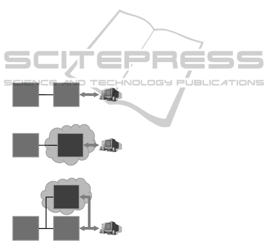
significant. The figure below provides a simplified
outline of the service environment.
Figure 1: Alternative service deployment scenarios.
For simplicity, the service is decomposed only
into two elements: the customer-facing element
responsible for information exchange with the
customers (e.g. a web-portal, a content-distribution
server, etc.) and the other subsystems
complementing the customer-facing element (e.g.
business logics, databases, etc.). It is assumed that
the interaction between the service side and the
customer side requires substantial volume of data to
be transferred, as depicted in the figure by using
bold solid lines.
The question is formulated as: Which of the three
alternatives incurs the minimum overall costs to the
provider of communication intensive services?
In order to answer this question, the total costs of
ownership (TCO) analysis is conducted. Namely, the
cost structure of the service infrastructure is
determined based on the available literature. After
that, the cumulative costs of setting up and operating
the service over the period of ownership are
estimated, and the results of the estimation are used
to compare alternatives.
The remainder of the paper is organized as
follows. The details of the cost structure used in the
TCO analysis are provided in Section 2. Section 3
describes how the individual cost factors can be
estimated. In Section 4, a mixture of in-house (not-
leased) and leased infrastructure is studied, in order
to identify a combination with minimum TCO. The
results of applying the model to assess the costs of a
university content management system are reported
in Section 5. Finally, concluding remarks are given
in Section 6.
2 TOTAL COST OF OWNERSHIP
To confront the limitations of a simplistic costs
analysis based on the acquisition price only, the total
costs of ownership (TCO) analysis has been
introduced as a systematic analytical tool for
understanding the total costs associated with
acquiring and using a good or service. The TCO
analysis covers the key cost constituents of pre-
acquisition, acquisition and possession, use, and
disposal (Ellram 1993; Ellram 1995).
A number of cost-drivers can be potentially
taken into account. For instance, Ferrin and Plank
(2002) report 237 cost drivers grouped into 13
categories. The choice of cost factors to be
considered depends on the particular industry:
transportation costs, for example, are vital in
logistics, whereas in the case of IT services these
costs might be ignored as less important. According
to David et al. (2002), the IT costs factors include
the acquisition, operations, and control costs – with
the latter being optional costs aimed at improving
the IT centralization and standardization, which in
turn results in reducing operations costs.
The costs relevant for the cloud-based services
are listed below; these were identified based on
Customer-
facing
element
CDN
Not-leased
Leased
Mixed
Other
sub-
systems
Customer-
facing
element
Other
sub-
systems
CDN
Customer-
facing
element
Other
sub-
systems
Customer-
facing
element
DEDICATED VS. ON-DEMAND INFRASTRUCTURE COSTS IN COMMUNICATIONS-INTENSIVE
APPLICATIONS
363

(David et al. 2002; Ferrin and Plank 2002; Murray
2007):
1. Pre-acquisition costs
- Costs of evaluating features and gap analysis
- SLA analysis, reviewing provider's security
2. Acquisition costs:
a. Infrastructure, software
- Hardware: servers, workstations, network and
security infrastructure
- Infrastructure and application software
b. Integration and deployment
- Requirements identification and software
configuration
- Integration software development or/and
acquisition
- Data conversion/migration
- User training
3. Operations costs:
a. External support
- Hardware support and maintenance
- Software support & maintenance
b. Fees for using on-demand (cloud) services
- Storage costs
- Data transfer costs
- Computing costs
c. Others
- Administering and operating the system
- Power consumption costs
- Facility (premises) maintenance and rent
- Training, auditing, downtime, security incidents
4. Control costs (centralization and standardization)
Table 1: Cost factors.
Cost
Own
deployment
Cloud
deployment
Mixed
Acquisition costs
Hardware
Software
Operations costs
Hardware support
& maintenance
Software support
and maintenance
Storage
Data transfer
Computing
Administering &
operating
Power
consumption
Facility
maintenance & rent
The premises are assumed to be leased rather then
owned; therefore, the costs of facility maintenance
and rent are estimated instead of the premise
acquisition costs. For simplicity, in what follows,
only acquisition and operations costs are considered,
whereas the pre-acquisition and control costs are
omitted. Furthermore, the integration and
deployment costs (2b) as well as some other cost
factors (namely, training, auditing, downtime, and
security incidents) for the sake of simplicity are
excluded from further consideration. The remaining
ones are collected in Table 1. Along with the cost
factors, the table contains the notations used for
these factors in three deployment scenarios.
3 COST FACTOR ESTIMATION
Ellram (1995) describes two approaches to TCO
evaluation: dollar-based and value-based
approaches. In dollar-based approach, either actual
cost of TCO constituents are used, or a formula is
applied to estimate the costs of each activity. Dollar-
based TCO analysis may be also based on formal
analytical models of pre- and post-acquisition costs:
mixed integer linear programming model (Degraeve
and Roodhooft, 1999); data envelope analysis
(Garfamy, 2006; Ramanathan, 2007). These
analytical models are particularly useful in supplier
selection for tangible assets, while their application
in the context of software products and services
appears challenging. The value-based approach is
used when costs cannot be directly quantified. In this
approach, costs are complemented with qualitative
performance indicators which are transformed to
quantitative values. Such transformation takes into
account weights of variables and requires significant
efforts for fine-tuning.
In this work, the dollar-based approach is
followed. Thus, for the purposes of the analysis, the
values of the factors should be either:
- estimated based on the real expenses as incurred in
the organization;
- approximated based on expert knowledge; or
- approximated based on the trends and reference
values reported in the literature.
Below, the cost estimation for the customer-facing
element of the service is discussed for all three
deployment scenarios. No cost estimation is done for
the rest of the service infrastructure, since it is
assumed to remain constant in all three scenarios
and hence will not affect the results of the
comparison.
CLOSER 2011 - International Conference on Cloud Computing and Services Science
364

3.1 “Own” Deployment Scenario
Let us assume that the “own” deployment is either
currently state-of-the-art, or are extensively
described in literature. Therefore, for this scenario, a
majority of variables can be estimated based on the
real expenses or based on the estimates found in the
literature.
It should be noted that storage fee (
) and
computing fee (
) are likely to be zero in this
scenario. Furthermore, hardware and software
maintenance costs can be approximated as a
percentage of the hardware and software
maintenance costs. For instance, yearly hardware
support costs can be assumed to be 20% of the
hardware acquisition costs (Murray 2007).
Thus, the variables to be assigned based on real
expenses/literature include the costs of hardware and
software acquisition (
,
), data transfer (
), as
well as the costs of administration/operating, power,
and facility costs (
,
,
). It should be noted that
the data transfer costs (
) reflect the charges paid to
a communication service provider for allocated
bandwidth, i.e. the high-bandwidth last-mile access
is assumed to be available.
Hardware acquisition costs (
). Nowadays,
many organizations utilize a virtualized
environment, wherein servers are implemented as
server instances running on virtual CPUs (vCPUs).
In such environment, multiple servers are sharing
the same underlying hardware, thus making it
difficult to estimate the costs of individual instances
directly. In order to address this problem, the vCPU
costs can be estimated as follows.
For each instance, its hardware requirements are
stated, and the number of vCPUs to fulfill these
requirements is estimated. Assuming homogeneous
vCPU, the number of vCPUs can be estimated as
vCPU
=max
m
m
,
d
d
,
c
c
,
(1)
Where
m
,
d
, and
c
are memory, disc space, and
computing resources of a single vCPU, and
m
,
d
,
and
c
are the requirements of an instance.
The cost of a single vCPU is estimated, by
aggregating the costs of virtualized hardware and
dividing it by the total number of virtual machines.
Finally, the server instance costs are estimated as a
product of the number of vCPUs needed and the
vCPU cost.
Software acquisition costs (
). Once the number of
vCPU is known, the costs of software licenses per
vCPU can be estimated. The total software
acquisitions costs are then a product of per-vCPU
software licenses costs and the number of vCPUs. It
should be noted that some of the software products
(such as the virtualization layer software) are
allocated to blades rather than to a vCPU, and
therefore their costs need to be accounted separately.
3.2 “Cloud” Deployment Scenario
The costs of hardware acquisition (
) and
maintenance (
) are zero in the “cloud” scenario.
Depending on the software used, the costs of
software licenses acquisition (
) and software
support (
) may be zero (the case of open source),
equal to the software costs in the “own” deployment
scenario (the same software is used in the cloud), or
in between. Also such a case can be envisioned,
where different (and more expensive) software
needs to be used in cloud due to the limitations of
the cloud platform; this case is not considered here.
The costs of storage, data transfer, and
computing depend both on the requirements of the
service, and on the pricing of the cloud infrastructure
providers. Specifically, based on the service
requirements, the offerings of multiple cloud
infrastructure providers are retrieved, the least
expensive offering meeting the requirements is
identified, and the corresponding values are used to
assign the values to the storage (
), data transfer
(
), and computing (
) costs.
Administering/operating costs (
) are roughly
equal to the administering/operating in the “own”
deployment scenario – the same personnel is
assumed to administer the service infrastructure,
whether it is deployed in-house or in the cloud.
Since no hardware is used, the power and facility
costs (
,
) are likely to be negligibly small and
are therefore assigned 0.
3.3 “Mixed” Deployment Scenario
In the mixed deployment scenario, a part of the
customer-facing element functionality is kept in
house, while the remainder is allocated to the cloud-
based infrastructure. This results in the following
changes, as compared with the two deployment
scenarios above.
First, data may need to be replicated in-house
and in the cloud. Depending on the specifics of the
service, it may be possible to divide the data among
in-house and cloud infrastructure, but for simplicity
it is assumed that complete replica of data needs to
be presented in both locations. Thus, the costs of
data storage (
) are equal to the data storage costs
in the “cloud” deployment scenario.
DEDICATED VS. ON-DEMAND INFRASTRUCTURE COSTS IN COMMUNICATIONS-INTENSIVE
APPLICATIONS
365

Second, a part of the data communication with
the customers is carried out in-house (by the in-
house customer-facing element), while the rest is
done by the cloud. Let (0≤≤1) denote the
portion of data transferred through the in-house
customer-facing element, and let denote the total
volume of the traffic. The data transfer costs
can
be represented as a function
(,); the details of
this function will be discussed below.
Finally, a part of computing is performed with
in-house (virtualized) infrastructure, while the rest is
performed in the cloud. Both the computing
demands and the volume of data transferred grow
proportionally with the number of customers served.
It is therefore reasonable to assume that portion of
computing power is assigned to the in-house
infrastructure, whereas the rest (i.e. 1−) is
assigned to the cloud.
Hardware Acquisition and Maintenance Costs. Only
the portion of the hardware deployed in-house incurs
costs. Therefore, the hardware costs
and
can be
estimated as
=
and
=
respectively.
Software Acquisition and Maintenance Costs. A
portion of software is used by the in-house
hardware, and the rest is used in the cloud. Since the
need for software licenses change with the vCPUs
used in-house and in the cloud, the software
acquisition costs can be estimated as
=
+
(
1−
)
;
(2)
=
+
(
1−
)
.
(3)
Data transfer costs. In total,
own
= bytes are
transferred through in-house infrastructure, and
cloud
=(1−) bytes of data are transferred
through the cloud. Let
own
(
own
) denote the price
of one byte of data transferred via in-house
infrastructure, and
cloud
(
cloud
) denote the price of
one byte transferred through the cloud. The volume
is included as a parameter in the brackets in order to
emphasize the fact, that the data transfer price per
byte depends (in fact, decreases with the growth of)
the overall volume. Then, the data communication
costs can be estimated as:
=
(
,
)
≡
own
own
(
own
)
+
cloud
cloud
(
cloud
)
.
(4)
The values of the cloud data transfer price
cloud
(
cloud
) can be derived from the offerings of
the cloud infrastructure providers. In order to
approximate the in-house data transfer costs, the
dependency between the data volume and the price
need to be determined. In this work, the following
function is used in order to approximate this
dependency:
=
,
(5)
where
and
are empirically estimated from
reference values. For instance, by using the
reference values from http://www.prospeed.net/, the
and
can be estimated as
= 112.77 and
= −0.22 respectively.
Computing costs. Only the computing performed in
the cloud incurs costs. Therefore, the computing
costs
can be estimated as
=(1−)
.
Administration/operating, power, and facility costs.
As in the “cloud” deployment, the same personnel
can be assumed to carry out the tasks, i.e.
=
.
The power and facility costs are assumed to be
proportional to the in-house computational load and
data transfer, which are manifested in the value,
i.e.
=
and
=
.
The estimators for different cost factors are
summarized in Table 2. The factors whose values
need to be assigned based on the real expenses or
literature are shown in bold; the majority of such
factors belong to the “own” deployment scenario.
The factors in the “cloud” deployment are assigned
based on the offerings of the cloud infrastructure
vendors. The other costs can then be derived from
these values.
The total costs of a deployment scenario are
estimated as a sum of the cost factors constituting
the scenario. It is assumed that the acquisition costs
are incurred only once, whereas the operations costs
are reoccurring on yearly basis. Then, for years of
ownership, the total costs are estimated for different
scenarios as:
own
=
+
;
(6)
cloud
=
+
;
(7)
mixed
=
+
.
(8)
4 COMPARING THE
DEPLOYMENT SCENARIOS
As described in the previous section, the costs in the
“mixed” deployment scenario depend on the value
of indicating how large portion of data transport
and computing is allocated to the in-house service
CLOSER 2011 - International Conference on Cloud Computing and Services Science
366

infrastructure. In fact, the “mixed” scenario can be
seen as a general case, with “own” and “cloud”
being the special cases for =1 and =0
respectively. In this section, the effect of on the
overall costs in the “mixed” deployment scenario is
studied, with the aim to identify the value of at
which the overall costs would be minimized.
In order to find the value of corresponding to
the minimum of
mixed
, the first and the second
derivatives of
mixed
are considered:
mixed
(
)
=
(
)
+
(
)
=
=
+
−
+ ×
(
+
−
+
(
,
)
−
+
+
)
(9)
In the beginning of the paper, we assumed that the
costs of network data transfer contributes the most to
the overall service cost structure, i.e.
=
(
,
)
≫
,
∈
1,2,3,4,5,7,8,9,10
.
(10)
Therefore, when evaluating the derivative
mixed
(),
it is reasonable to focus on the term
(
,
)
, while
the remaining part can be substituted with a constant
:
mixed
(
)
=
(
,
)
+
. (11)
As described in the previous section, the function
(
,
)
is defined as
(
,
)
=
+
(
1−
)
×
cloud
(
1−
)
.
(12)
Let us assume that the pricing of a cloud
infrastructure provider can as well be represented as
a power function of the volume:
cloud
=
cloud
.
(13)
The function
(
,
)
can now be rewritten as:
(
,
)
=
(
)
+
(
1−
)
(
(
1−
)
4=
1
1+
2+
3(
−
)1+
4.
(14)
Then, the derivative
mixed
(
)
is:
mixed
(
)
=×
[
(
1+
)(
)
+
(1 +
)
×(−)
(−)
]
=
[
(
1+
)(
)
−
(1 +
)( − )
]
.
(15)
The function
mixed
has an excess when
mixed
(
)
=
0, i.e. when
(
1+
)(
)
=
(1 +
)( − )
.
(16)
When
=
and
=
, it follows that
mixed
(
)
=0, when =0.5.
Similarly, the second derivative
mixed
(
)
can be
evaluated as
mixed
(
)
=×
[
(
1+
)
(
)
+
(1 +
)
(
−)
]
>0.
(17)
The second derivative is positive for all values of
∈[0,1]. Thus, the function
mixed
(
)
is concave,
and hence the minimum of the costs is achieved at
one of the boundary values: =0 or =1. Which
of them corresponds to the minimum costs depends
on the values of the coefficients
,
,
, and
, as
well as on the interplay of other costs (encompassed
by the constant ). Therefore, in case the data
transfer costs dominate in the service infrastructure
cost structure, either “in-house” or “cloud”
deployment options are cost-optimal, whereas higher
costs are going to be incurred with the “mixed”
deployment.
Table 2: Cost estimation.
Cost “Own” deployment “Cloud” deployment “Mixed” deployment
Acquisition costs
Hardware
0
=
Software
=
+
(
1−
)
Operations costs
Hardware support and maintenance
=
0
=
Software support and maintenance
=
0
=
+
(
1−
)
Storage
0
=
Data transfer
=
(,)
Computing
0
=(1−)
Administering/operating
=
=
Power consumption
0
=
Facility maintenance/rent
0
=
DEDICATED VS. ON-DEMAND INFRASTRUCTURE COSTS IN COMMUNICATIONS-INTENSIVE
APPLICATIONS
367

5 CASE STUDY:
A UNIVERSITY CONTENT
MANAGEMENT SYSTEM
In this section, the costs of deployment options are
compared for the case of university content
management system based on Plone.
In this case, the “own” deployment assumes the
acquisition of a Dell PowerEdge M610 server, and
installing a stack of open-software on it, including
Zope WWW-application server, Zope Object
Database, Zope Enterprise Objects, Plone content
management system, etc. (Ojaniemi 2010). The costs
of hardware acquisition are estimated based on the
price of the server as €4102. The current outbound
data transfer volume is estimated at the order of
1TB/month, which, assuming the price of $0.11
(€0.078) per GB, corresponds to the costs of €80.
In future, with the increased proliferation of
online teaching content, the data transfer volume
may increase dramatically by the factor of 100, thus
reaching 100TB/month and resulting in the monthly
data transfer costs of €8023. On the other hand, in a
hypothetical case of shifting the content
provisioning to individual departments’
infrastructure, the data volume of the university
content management system may be decreased
tenfold to 0.1TB/month, resulting in the data transfer
costs of €8/month.
In the “cloud” deployment scenario, the
computing requirements of the current service are
assumed to be met by EC2 extra large instance. With
the Amazon pricing, the data transfer costs for the
current load are €109.4/month; in case of the
increase to 100TB/month, the data transfer cost will
rise to €7720.5/month; in case of the downscaling to
0.1TB/month, the cost will drop to €10,9/month.
When the load increases by the factor of , the
number of requests to the server(s) is also going to
increase, but at a smaller pace, e.g. the by the factor
of
√
– reflecting the assumption that the increase in
load due to new type of content rather than new
students. Then, the increased load would need to be
served by
√
in-house servers (“own” deployment)
or by
√
extra large instances (“cloud” deployment).
Based on Amazon pricing, the computing costs
for the current service in “cloud” deployment
comprise €222/month. For the increased load, the
costs would rise to €2218. For the decreased load,
the smaller computing power is required; assuming
that the Amazon Large instance is sufficient, the
monthly computing costs would decrease to
€111/month.
For “own” deployment, the maintenance costs
for the acquitted hardware are assumed to be 20% of
the acquisition price. The other costs (including the
costs of storage needed) are either assumed equal for
both alternatives, or are assumed negligible.
The resulting costs are summarized in the table
below, and the computing, bandwidth, and total
costs accumulated over 3 years are visualized in
Figure 2. As could be seen from the table, as soon as
the data transfer costs represent the major cost
constituent (which is the case with the increased data
transfer), the “cloud” deployment option is less
expensive than the “own” deployment. Furthermore,
according to the discussion in the previous section,
the cost of “mixed” scenario will be greater than the
“cloud” deployment’s costs in this case.
For the case with the current and the decreased
data transfer, the contribution of the data transfer to
the total costs is more significant. As a consequence,
the result of the comparison is different: the “cloud”
deployment option is more expensive. Primarily, this
is due to the high costs of Amazon instances.
6 CONCLUSIONS
In this paper, a quantitative model for assessing the
total costs of alternative software deployment
options has been introduced, whereby the costs of
Table 3: Costs of the university management system.
Costs Current data transfer Increased data transfer Decreased data transfer
“Own” “Cloud” “Own” “Cloud” “Own” “Cloud”
Acquisitions 4 102,9 € 0,0 € 41 028,6 € 0,0 € 1 296,5 € 0,0 €
Computing 820,6 € 2 661,3 € 8 205,7 € 26 613,5 € 259,3 € 1 330,7 €
Data transfer 962,7 € 1 312,8 € 96 273,5 € 86 646,2 € 96,3 € 131,3 €
Total 1st year 5 886,2 € 3 974,2 € 145 507,8 € 113 259,6 € 1 652,1 € 1 462,0 €
Total 2nd year 7 669,5 € 7 948,3 € 249 987,0 € 226 519,3 € 2 007,7 € 2 923,9 €
Total computing 6 564,6 € 7 984,0 € 65 645,8 € 79 840,5 € 2 074,5 € 3 992,0 €
Total data transf. 2 888,2 € 3 938,5 € 288 820,5 € 259 938,5 € 288,8 € 393,8 €
Total 3rd year 9 452,8 € 11 922,5 € 354 466,3 € 339 778,9 € 2 363,3 € 4 385,9 €
CLOSER 2011 - International Conference on Cloud Computing and Services Science
368
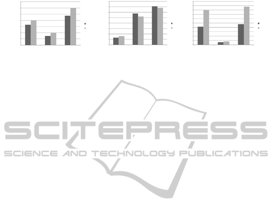
a) Current load b) Increased load c) Decreased load
Figure 2: Comparing the computing, bandwidth, and total costs accumulated over three years for the “own” and the “cloud”
deployments.
in-house service infrastructure can be compared with
the cost of cloud-based infrastructure. Relevant cost
factors for the model have been identified. Some of
these factors are to be estimated based on the real
expenses of expert opinion, while for the others,
their values are derived from the already assigned
variables.
The costs of the mixed scenario, wherein the
computing and data transfer load is distributed
between the in-house and cloud infrastructure have
been analytically analyzed. According to the
obtained results, either the “in-house” or the “cloud”
deployment options, but not the “mixed”
deployment are cost-optimal whenever the data
transfer costs represent the major component of the
infrastructure costs.
The usual assumption of mixed cloud being cost-
effective in combining less expensive stable in-
house capacity with use of cloud for handling
demand peaks (Weinman 2009a) seems to be a
somewhat limited view. That is, the assumption
seems to hold mainly in computing intensive
applications, where the additional relevant cost,
including network bandwidth costs, are minor and
hence can be ignored. Meanwhile, communication
intensive applications are most cost-effective in a
single point of service, which can make use of
economy of scale in purchasing communication
capacity. For these communication intensive cases,
the mixed cloud solution has to bear the costs of two
smaller communication pipes (for in-house and for
the cloud), thus enforcing the use of higher costs of a
unit of bandwidth applied to smaller capacity. Even
if the communication cost between the in-house
implementation and the cloud site neglected, such a
mixed cloud is likely to be more expensive than the
single point of service (Weinman 2009b).
This work has focused on costs of the
communication intensive applications. Further work
will still be needed to analyze costs related to
various combinations of processing, data and
communication intensive cases in mixed clouds.
ACKNOWLEDGEMENTS
This research reported in this paper was carried out
in the frame of the Cloud Software Program of the
Strategic Centre for Science, Technology and
Innovation in the Field of ICT (TIVIT Oy) funded
by the Finnish Funding Agency for Technology and
Innovation (TEKES).
REFERENCES
David, J. S., Schuff, D., and Louis, R. St. (2002),
Managing your IT Total Cost of Ownership,
Communications of the ACM, 45 (1), 101-106.
Degraeve, Z. and Roodhoft, F. (1999b), Improving the
efficiency of the purchasing process using total cost of
ownership Information: The case of heating electrodes
at Cockerill Sambre S. S. European Journal of
Operational Research, 112, 42-53.
Ellram, L. M. (1993), A framework for Total Cost of
Ownership, the International Journal of Logistics
Management 4(2), pp. 49-60.
Ellram, L. M. (1995), Total cost of ownership: An analysis
approach for purchasing, International Journal of
Physical Distribution & Logistics Management, 25
(8), pp. 4-23.
Garfamy, R. M. (2006), A data envelopment analysis
approach based on total cost of ownership for supplier
selection. Journal of Enterprise Information
Management, 19, 662-678.
Lee, C. A. (2010), A perspective on scientific cloud
computing. In Proceedings of the 19th ACM
International Symposium on High Performance
Distributed Computing (HPDC '10). ACM, New
York, NY, USA, 451-459.
Luoma, E., Mazhelis, O., and Paakkolanvaara, P. (2010),
Software-as-a-Service in the telecommunication
industry: Problems and opportunities. In the
Proceedings of the first International Conference on
Software Business (ICSOB2010), University of
Jyväskylä, Finland, June 21-23, pp. 138-150.
Mazhelis, O., and Tyrväinen, P. (Eds.) “Vertical Software
Industry Evolution: Analysis of Telecom Operator
-€
2 000,0 €
4 000,0 €
6 000,0 €
8 000,0 €
10 000,0 €
12 000,0 €
14 000,0 €
Total computing Total data transfer Total 3rd year
Own
Cloud
-€
50 000,0 €
100 000,0 €
150 000,0 €
200 000,0 €
250 000,0 €
300 000,0 €
350 000,0 €
400 000,0 €
Total computing Total data transfer Total 3r d ye ar
Own
Cloud
-€
500,0 €
1 000,0 €
1 500,0 €
2 000,0 €
2 500,0 €
3 000,0 €
3 500,0 €
4 000,0 €
4 500,0 €
5 000,0 €
Total computing Total data transfer Total 3rd year
Own
Cloud
DEDICATED VS. ON-DEMAND INFRASTRUCTURE COSTS IN COMMUNICATIONS-INTENSIVE
APPLICATIONS
369

Software”, Contributions to Management Science
Series, Springer, 2009.
Murray, Andrew Conry (2007), TCO Analysis: Software
as a Service, United Business Media, March 2, 2007,
available online at http://www.networkcomputing.
com/other/tco-analysis-software-as-a-service.php
(last retrieved on November 3, 2010)
Ojaniemi, J. (2010), Pilvipalveluiden käyttöönotto - edut,
haasteet ja kustannukset, M.Sc. Thesis, University of
Jyväskylä, Finland.
Ramanathan, R. (2007), Supplier Selection problem:
Integrating DEA with the approaches of total cost of
ownership and AHP. Supply Chain Management: An
International Journal, 12, 258-261.
Tyrväinen, P., Warsta, J. and Seppänen (2008), V.:
Evolution of Secondary Software Businesses:
Understanding Industry Dynamics, in IFIP
International Federation for Information Processing,
Vol. 287, Open IT-Based Innovation: Moving
Towards Cooperative IT Transfer and Knowledge
Diffusion, eds. León, G., Bernardos, A., Casar, J.,
Kautz, K., and DeGross, pp. 381-401. Springer.
Weinman, J. (2009a), Mathematical Proof of the
Inevitability of Cloud Computing, Cloudonomics.com,
available online at http://cloudonomics.wordpress.com/
(last retrieved on November 8, 2010).
Weinman, J. (2009b), 4 1/2 Ways to Deal With Data
During Cloudbursts, GigaOm, available online at
http://gigaom.com/2009/07/19/4-12-ways-to-deal-with
-data-during-cloudbursts/ (last retrieved on November
8, 2010).
Youseff, L., Butrico, M., and Da Silva, D. (2008), Toward
a Unified Ontology of Cloud Computing, Grid
Computing Environments Workshop (GCE '08), pp.
1-10.
CLOSER 2011 - International Conference on Cloud Computing and Services Science
370
