MONOCULAR RECTANGLE RECONSTRUCTION
Based on Direct Linear Transformation
Cornelius Wefelscheid, Tilman Wekel and Olaf Hellwich
Computer Vision and Remote Sensing, Berlin University of Technology
Sekr. FR3-1, Franklinstr. 28/29, D-10587, Berlin, Germany
Keywords:
Rectangle, Quadrangle, Reconstruction, Direct linear transformation, Single view, Perspective projection.
Abstract:
3D reconstruction is an important field in computer vision. Many approaches are based on multiple images
of a given scene. Using only one single image is far more challenging. Monocular image reconstruction can
still be achieved by using regular and symmetric structures, which often appear in human environment. In
this work we derive two schemes to recover 3D rectangles based on their 2D projections. The first method
improves a commonly known standard geometric derivation while the second one is a new algebraic solution
based on direct linear transformation (DLT). In a second step, the obtained solutions of both methods serve as
seeding points for an iterative linear least squares optimization technique. The robustness of the reconstruction
to noise is shown. An insightful thought experiment investigates the ambiguity of the rectangle identification.
The presented methods have various potential applications which cover a wide range of computer vision topics
such as single image based reconstruction, image registration or camera path estimation.
1 INTRODUCTION
The research field of 3D reconstruction has been stud-
ied intensively in the last years. The majority of cur-
rent reconstruction techniques rely on at least two im-
ages from different perspectives to compute the depth
of a scene (Hartley and Zisserman, 2003). This topic
is referred as structure from motion (Faugeras and
Lustman, 1988) which can be solved by the five point
algorithm (Nister, 2004) or simultaneous localization
and mapping (SLAM) approaches (Davison et al.,
2007).
Although recovering 3D information based on
one image is mathematically impossible, it has been
shown that humans are able to perceive the 3D shape
of an object based on monocular images. The exam-
ple in Fig. 1 shows that the drawing of a Necker cube
is perceived as a 3D object rather than an arrange-
ment of lines in 2D space. Prior knowledge about
the given scene allows us to interpret this figure cor-
rectly as a projection of a known 3D geometry and we
do not rely on multiple perspectives. The rectangular
structure as well as the symmetry of a cube is used as
apriori-information. We implicitly assume that a cube
is more likely to see than an arbitrary arrangement
of lines. Pizlo (Pizlo, 2008) shows that 3D informa-
tion obtained from single images in combination with
prior knowledge is more reliable and robust than 3D
information from stereo. Psychology has investigated
the shape constancy and the shape ambiguity problem
(Todd, 2004). The shape constancy problem raises
the question whether two different 2D views could be
yielded by the same 3D object. The shape ambiguity
problem deals with the question whether the same 2D
view is induced by either the same or two different
3D objects. For an engineering-oriented investigation
both are substantial: (1) The shape constancy prob-
lem presumes that a 3D shape can be inferred from
monocular images. (2) The shape ambiguity problem
forbids to trust a solution that is based on a single im-
age. Among many other geometrical models, rectan-
gular structures are of particular interest. Many ob-
jects in our environment are characterized by rectan-
gles such as doors, windows or buildings. The math-
ematical description as well as the detection is rela-
tively easy which is very important in practice. This
work presents two approaches for the reconstruction
of a 3D rectangle from its 2D perspective projection
on a single image plane. We discuss the problem of
shape constancy and shape ambiguity from a percep-
tual viewpoint and provocatively hypothesize that all
perspectively distorted quadrangles look like rectan-
gles, which is supported by an experimental setup at
the end of this paper. This paper is organized as fol-
271
Wefelscheid C., Wekel T. and Hellwich O..
MONOCULAR RECTANGLE RECONSTRUCTION - Based on Direct Linear Transformation.
DOI: 10.5220/0003317502710276
In Proceedings of the International Conference on Computer Vision Theory and Applications (VISAPP-2011), pages 271-276
ISBN: 978-989-8425-47-8
Copyright
c
 2011 SCITEPRESS (Science and Technology Publications, Lda.)

Figure 1: Image of a Necker cube.
lows. In the next section we present related work and
emphasize the differences compared to our approach.
Two mathematical methods are derived in Section 3.
Here, we present an improved and simplified version
of the approach presented in (Haralick, 1989) before
we introduce a new method based on DLT. The iden-
tification problem as well as the accuracy analysis are
discussed in Section 4. The proposed methods are
evaluated on real world data before the paper con-
cludes with an outlook to future work.
2 PREVIOUS WORK
Using rectangular structures to compute various infor-
mation such as calibration and orientation of the cam-
era is not new. Different approaches for single im-
age based reconstruction have been presented in the
past. All of them rely on several constraints such as
parallelism and orthogonality in order to retrieve the
missing information (Wilczkowiak et al., 2001). Van-
ishing points are used to compute the internal and ex-
ternal parameters of a camera (Sturm and Maybank,
1999). The computation tends to become unstable
since these points are often placed near infinity. The
work presented in (Haralick, 1989) is partly similar
to our approach. It presents different derivations han-
dling degenerated scene configurations such as copla-
narity. This is not mandatory as it can be seen in Sec-
tion 3. In contrast to previous efforts, we introduce a
novel method which solves the stated problem by us-
ing a standard DLT method. In (Delage et al., 2007),
Markov random fields (MRF) are used for detecting
different planes and edges to form a 3D reconstruc-
tion from single image depth cues. In contrast to our
work they assume orthogonal planes instead of deal-
ing with the rectangle structure itself. (Micusk et al.,
2008) describes an efficient method for detecting and
matching rectilinear structures. They use MRF to la-
bel detected line segments. This approach enables the
detection of rectangles even if the four line segments
are not detected accurately. In (Lee et al., 2009), the
scene is reconstructed by building hypotheses of in-
tersecting line segments.
3 DERIVATION
We present two methods for reconstructing a rectan-
gle in 3D space. The first method is based on ge-
ometric relations while the second one is a new al-
gebraic solution. We assume a calibrated camera in
both cases. In this context we are only interested in
quadrangles with a convex shape since the projection
of a rectangle is never concave. Our primary goal is
to compute the orientation and the aspect ratio of a
rectangle in 3D space from a perspectively distorted
2D image of a rectangle. This is equivalent to the
computation of the extrinsic parameters of the cam-
era, e.g. in the local coordinate system defined by the
sides of the rectangle. The secondary goal is to verify
that the observed quadrangle is yielded by a rectangle
in 3D space and not by any other planar quadrangle.
We have to exclude as many non-rectangular quad-
rangles as possible from further processing early and
efficiently. The theoretical aspects of this problem are
discussed in Section 4.
3.1 Geometric Method
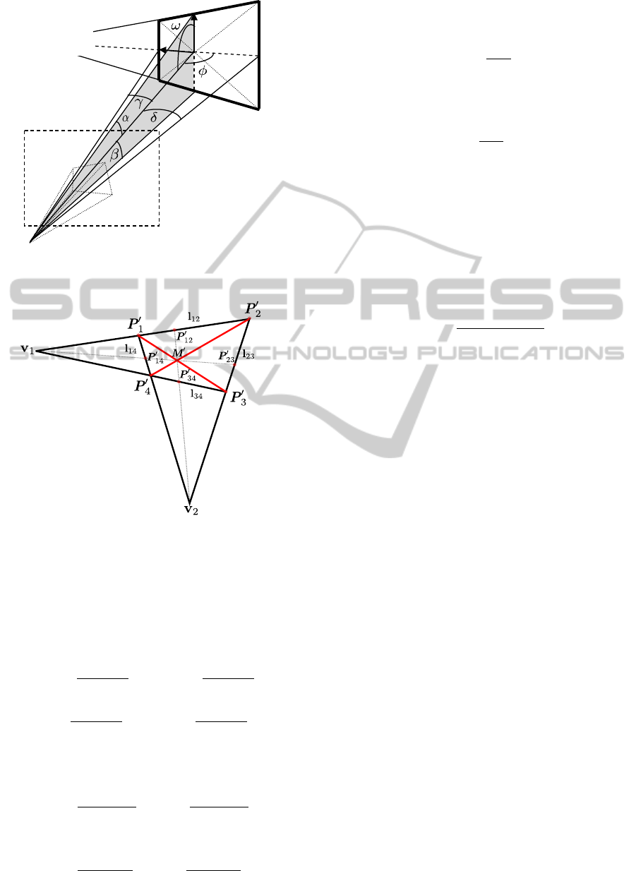
Fig. 2 shows the arrangement of a 3D rectangle pro-
jected onto an image plane and Fig. 3 contains the 2D
image representation. For the sake of clarity, we con-
sider a camera that is placed in the origin and looks
in Z-direction. P
1
...P
4
are the corner points of the
rectangle and p
0
1
...p
0
4
are the corresponding projec-
tions in the image plane of the camera. They can be
expressed in homogeneous coordinates p
0
1
...p
0
4
. Ne-
glecting the intrinsic camera parameters, the points
p
0
i
are transformed to P
0
i
, which are the corner points
of the rectangle’s projection in the world coordinate
system. They are connected by the edges of the rect-
angle l
12
, l
14
, l
23
and l
34
. Opposing edges intersect
at the vanishing points v
1
and v
2
. The center point
M is defined as the intersection of the rectangle’s di-
agonals. M
0
is the projection of the center point M.
The line defined by v
1
and M
0
intersects the rectan-
gle’s edges at its centers P
0
14
and P
0
23
, respectively.
P
0
12
and P
0
34
are defined by the second vanishing point
v
2
. The points P
i
and the camera rotation angles ω,
φ and κ are deduced from the corner points P
0
i
. The
distance d from projection center to rectangle center
can be chosen arbitrarily. In the following we derive
the computation of a rectangle based on a quadrangle.
According to Figs. 2 and 3 we can derive the follow-
ing simple equations:
l
i j
= P
0
i
× P
0
j
(1)
M
0
= l
13
× l
24
(2)
v
1
= l
12
× l
34
v
2
= l
14
× l
23
(3)
VISAPP 2011 - International Conference on Computer Vision Theory and Applications
272

d
O
u
v
to v
1
image plane
Figure 2: 3D arrangement of camera and 3D rectangle.
Figure 3: 2D image of a rectangle.
P
0
12
= (v
2
× M
0
) × l
12
P
0
34
= (v
2
× M
0
) × l
34
P
0
23
= (v
1
× M
0
) × l
23
P
0
14
= (v
1
× M
0
) × l
14
(4)
α = arccos
P
0
T
12
M
0
|P
0
12
||M
0
|
,β = arccos
P
0
T
34
M
0
|P
0
34
||M
0
|
γ = arccos
P
0
T
14
M
0
|P
0
14
||M
0
|
,δ = arccos
P
0
T
23
M
0
|P
0
23
||M
0
|
.
(5)
Given all angles in the presented setup, the descrip-
tion of the points in space is straight forward:
|P
12
| =
2dsin(β)
sin(α + β)
,|P
34
| =
2dsin(α)
sin(α + β)
(6)
|P
14
| =
2dsin(δ)
sin(δ + γ)
,|P
23
| =
2dsin(γ)
sin(δ + γ)
. (7)
P
i j
are the center points of the edges defined by P
i
and P
j
:
P
i j
= |P
i j
|
P
0
i j
|P
0
i j
|
.
(8)
The rectangle is parametrized by the center point M
and the spanning vectors u and v,
M = d
M
0
|M
0
|
(9)
u = P
12
− M
v = P
14
− M .
(10)
The corner points of the rectangle can now be calcu-
lated as
P
1
...P
4
= M ± v ± u .
(11)
The equations derived above yield the following for-
mula for ω:
ω = arctan
2
cot(β) − cot(α)
.
(12)
The formula for φ and κ can be derived analogously.
3.2 DLT Method
The second method utilizes the well known DLT in
order to compute the parameters of the 3D rectangle.
In the following we define a linear system of 15 equa-
tions:
P
0
1
× (M + v + u) = 0
P
0
2
× (M − v + u) = 0
P
0
3
× (M − v − u) = 0
P
0
4
× (M + v − u) = 0
M
0
× M = 0 .
(13)
Each term in Eq. 13 yields only two linearly indepen-
dent equations. We compose a design matrix (A|B)
which is solved for (M
x
,u
x
,v
x
,M
y
,u
y
,v
y
,M
z
,u
z
,v
z
)
using Singular Value Decomposition (SVD):
(A|B) · (M
x
,u
x
,v
x
,M
y
,u
y
,v
y
,M
z
,u
z
,v
z
)
T
= 0 . (14)
The design matrix (A|B) is defined as followed:
A =















1
T
0
T
0
T
-1
T
1 -1 1 0
T
0
T
-1 1 -1
1 -1 -1 0
T
0
T
-1 1 1
1 1 -1 0
T
0
T
-1 -1 1
1 0 0 0
T
0
T
-1 0 0















(15)
MONOCULAR RECTANGLE RECONSTRUCTION - Based on Direct Linear Transformation
273

B =
















-P
0
1,x
-P
0
1,x
-P
0
1,x
P
0
1,y
P
0
1,y
P
0
1,y
-P
0
2,x
P
0
2,x
-P
0
2,x
P
0
2,y
-P
0
2,y
P
0
2,y
-P
0
3,x
P
0
3,x
P
0
3,x
P
0
3,y
-P
0
3,y
-P
0
3,y
-P
0
4,x
-P
0
4,x
P
0
4,x
P
0
4,y
P
0
4,y
-P
0
4,y
-M
0
x
0 0
M
0
y
0 0
















, (16)
where the subindex x, y or z indicates the coordinate
of the corresponding point or vector. Using the pre-
sented equations, we always compute parallelograms.
We can formulate an additional condition to check if
the detected shape is a rectangle:
• The angle between the spanning vectors u and v
must be perpendicular, so it must hold u
T
v = 0.
The condition is satisfied by rectangles only.
3.3 Optimization
If noise is taken into account we try to find a rectangle
which sufficiently approximates the observed quad-
rangle. We limit the parametrization to eight degrees
of freedom in order to assure the orthogonality of the
spanning vectors. It turns out to be reasonable to ex-
clude v
x
or v
y
from the parameter set. Both values v
x
or v
y
are then computed out of u, v
y/x
, and v
z
such that
u and v are perpendicular.
v
x
= -
u
y
v
y
+ u
z
v
z
u
x
(17)
Omitting v
z
would lead to a division by zero if the
rectangle is coplanar to the image plane. This cannot
occur for v
x
or v
y
because the image plane would be
perpendicular to the rectangle.
In this case the projection of the rectangle is a line
rather than a quadrangle. The computed rectangle is
still not optimal because the spanning vectors are only
close to be perpendicular. If we are only interested in
the orientation and ratio of the rectangle, a parallelo-
gram will already be a good approximation. We min-
imize the reprojection error defined in Eq. 18 in order
to get the optimal solution. P
r
and P
q
is a set of cor-
ner points. The index r represents the back projected
rectangle whereas q is the measured quadrangle.
min
4
∑
i=1
dist(P
0
ri
,P
0
qi
)
2
(18)
This minimization is done using the Levenberg-
Marquardt-algorithm. The algorithm shows a good
convergence behavior if the obtained parallelogram
parameters are used as seeding points. The optimiza-
tion as well as the proposed methods are analyzed on
synthetic and real world data in the following sec-
tions.
4 EXPERIMENTS
In this section we want to discuss the ambiguity of
the rectangle identification. Each quadrangle in an
image can be perfectly restored to a parallelogram in
3D space. According to the derivation in section 3.1,
this reconstruction is unique up to a scale factor. In
practice we have to deal with the presence of noise.
In this section, we investigate this problem in two ex-
periments: 1. Is it possible to distinguish between a
parallelogram and a rectangle? 2. How accurate is the
restoration of a noisy rectangle?
We define LE to be the length of the longest edge of
the quadrangle and normalize all errors to make them
invariant to the image size.
4.1 Identification
If we detect a quadrangle in an image we do not know
if this is a projection of a rectangle or just a parallel-
ogram. To examine this problem, we create arbitrary
parallelograms by randomly choosing uniformly dis-
tributed spanning vectors. Since we do not want to in-
vestigate the scaling, u and v have a constant length.
The ratio between u and v is a sample drawn from a
uniform distribution between 0.01 and 1.0. We create
10.000 parallelograms in total. A rectangle is com-
puted for each parallelogram minimizing the repro-
jection error as presented in Section 3.2 and 3.3. The
resulting projection error could either be caused by
noise or our assumption of measuring a rectangular
structure in 3D space is violated. If no prior knowl-
edge of the scene is given it is impossible to identify
the specific source of error. This question definitely
depends on the accuracy of the quadrangle detector.
The results presented in Fig. 4 show that after pro-
jective distortion it is not possible to distinguish be-
tween a 3D parallelogram and a 3D rectangle. As
the cumulative histogram presents, 90 percent of all
randomly created parallelograms have a distance of
less than 0.05 LE to the closest 3D rectangle. For
the sake of clarity we give a numeric example: If the
longest edge of a quadrangle is 50 pixels long, and a
quadrangle detector has an accuracy of σ = 2.5 pix-
els, 90 percent of all parallelograms are misperceived
as a rectangle. Based on the geometric appearance
only, it is not possible to distinguish reliably between
a parallelogram and a rectangle.
VISAPP 2011 - International Conference on Computer Vision Theory and Applications
274

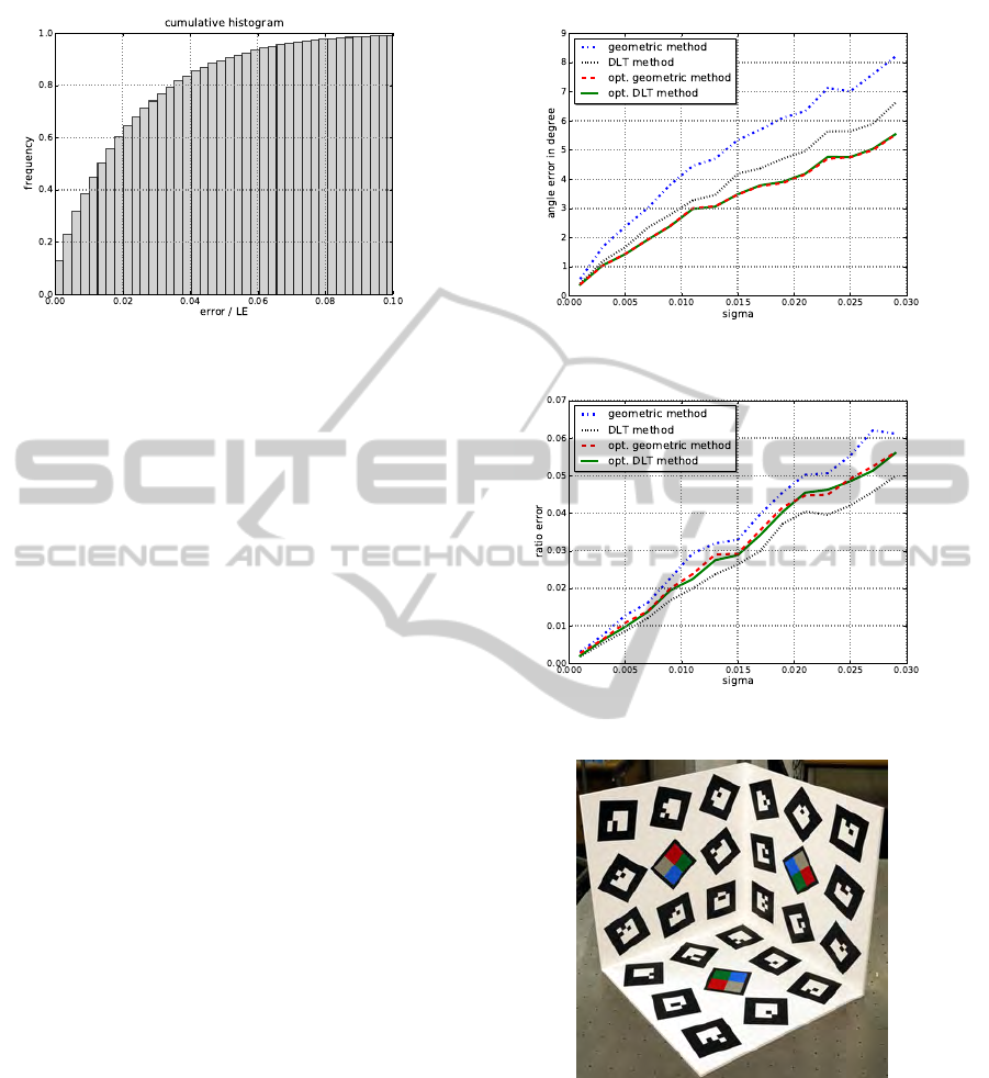
Figure 4: Cumulative histogram of the average error be-
tween original and calculated corner points of the quadran-
gle.
4.2 Accuracy
In contrast to the identification experiments, we eval-
uate the accuracy of the reconstructed rectangle in the
following. The most important quantities are the ra-
tio and the normal vector of the rectangle. Similar to
the experiment in 4.1, we randomly create 3D rect-
angles. Now, the spanning vector v is perpendicular
to u. We add normally distributed noise to the corner
points of the 2D quadrangle given by σ
px
= σ · LE.
We plot the average error of 1000 rectangles for dif-
ferent sigmas between 0.001 and 0.03. The angle and
ratio errors with respect to the original rectangle are
shown in Fig. 5 and Fig. 6 respectively. As it can be
seen in the figures, the error increases almost linearly
with the pixel noise. Nevertheless the methods deliver
good results even at high noise ratios.
5 RESULTS
In this section we evaluate the described methods on
real world data. We choose an object which has been
precisely measured by a laser scanner in order to pro-
vide ground truth. The cube shown in Fig. 7 contains
27 markers with different orientations. Nine mark-
ers are placed on each side. All three planes are per-
pendicular to each other. The colored markers in the
center of each plane are ignored and we get 24 rect-
angles in total. Fig. 8 and Fig. 9 show the reconstruc-
tion of the mentioned object and the corresponding
ground truth for a better illustration. In this example
the distance is of all rectangles is set to ground truth
to find a common scale. Using a calibrated camera
(12 mega-pixel), we have taken five images of the ob-
ject from different perspectives. We want to analyze
the aspect ratio and the orientation of each marker.
Figure 5: Angle error for different sigmas.
Figure 6: Ratio error for different sigmas.
Figure 7: Calibration object used for evaluation.
The corner points are precisely measured and we can
directly compare the ratio of each marker to ground
truth. For evaluating the angle error, we set the co-
ordinate system to the upper left corner of the first
maker. The computed angle should be either zero or
90 degree. The difference to the closest value is de-
fined as reconstruction error. The mean errors as
well as the standard deviations are presented in Ta-
ble 1 and Table 2. The resulting error is relatively
MONOCULAR RECTANGLE RECONSTRUCTION - Based on Direct Linear Transformation
275

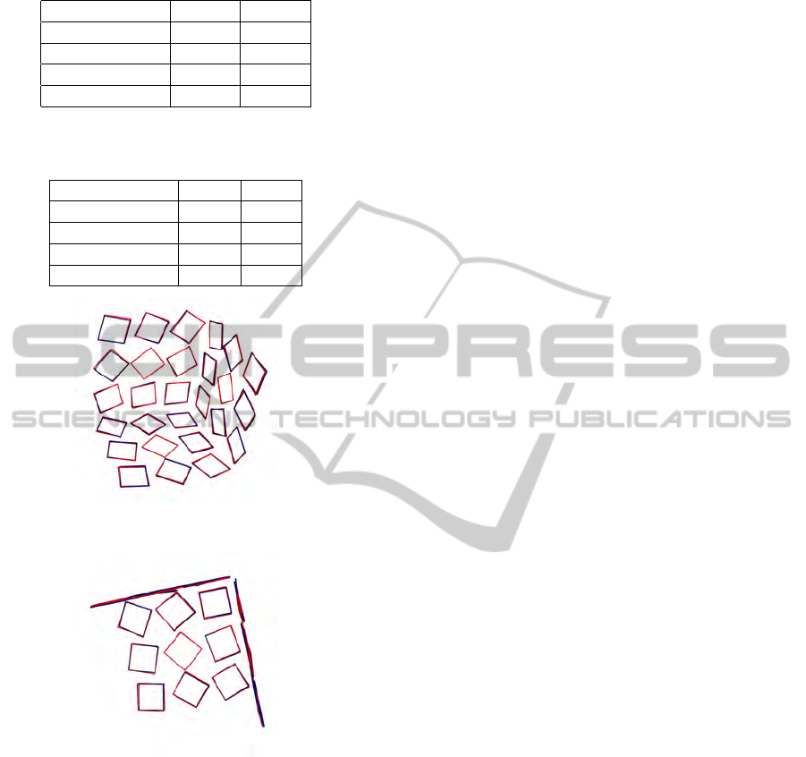
Table 1: Mean and standard deviation of the ratio error.
Ratio Mean Std.
Geometric 0.0123 0.0135
DLT 0.0123 0.0135
Opt. geometric 0.0119 0.0128
Opt. DLT 0.0114 0.0123
Table 2: Mean and standard deviation of the angle error in
degree.
Angle Mean Std.
Geometric 1.503 1.550
DLT 1.502 1.550
Opt. geometric 1.122 1.311
Opt. DLT 1.116 1.308
Figure 8: Reconstruction of the image in Fig. 7 marked in
blue and the ground truth measured with a laser scanner
marked in red.
Figure 9: The top view of the reconstruction shows the pre-
cise reconstruction. Only small errors can be seen in the
ground plane.
low. The evaluation on real world data show the same
characteristics as the simulation. In both cases the op-
timization improves the angle accuracy but shows less
effect on the ratio. Regarding the experiment in Sec-
tion 4.2, we can assume that the quadrangle detector
has a high accuracy.
6 CONCLUSIONS
We have presented two methods to compute a 3D
rectangle from a 2D quadrangle. The given results
show that the methods are stable even when applied
to noisy data. They can be utilized for further ap-
plications which could use rectangles as meaningful
shapes. These higher order shapes can improve the
accuracy in many computer vision tasks e.g. camera
calibration, orientation and path estimation. Monoc-
ular SLAM algorithms can be significantly improved
by using rectangles as landmarks. The initialization
of new rectangles from a single view and the estima-
tion of their depth improves the stability of such meth-
ods. In future work we will try to derive a method that
enables an analytic error propagation from the pixel
coordinates to 3D space. This maximizes the bene-
fit of rectangle based models in an extended Kalman
filter.
REFERENCES
Davison, A. J., Reid, I. D., Molton, N. D., and Stasse, O.
(2007). MonoSLAM: real-time single camera SLAM.
IEEE Transactions on Pattern Analysis and Machine
Intelligence, 29(6):1052–1067.
Delage, E., Lee, H., and Ng, A. (2007). Automatic single-
image 3d reconstructions of indoor manhattan world
scenes. Robotics Research, pages 305–321.
Faugeras, O. D. and Lustman, F. (1988). Motion and Struc-
ture From Motion in a Piecewise Planar Environment.
Intern. J. of Pattern Recogn. and Artific. Intelige.,
2(3):485–508.
Haralick, R. M. (1989). Determining camera parameters
from the perspective projection of a rectangle. Pattern
Recognition, 22(3):225–230.
Hartley, R. and Zisserman, A. (2003). Multiple view geom-
etry in computer vision. Cambridge University Press
New York, NY, USA.
Lee, D. C., Hebert, M., and Kanade, T. (2009). Geomet-
ric reasoning for single image structure recovery. In
IEEE Computer Society Conference on Computer Vi-
sion and Pattern Recognition (CVPR).
Micusk, B., Wildenauer, H., and Kosecka, J. (2008). Detec-
tion and matching of rectilinear structures. In CVPR.
IEEE Computer Society.
Nister, D. (2004). An efficient solution to the five-point
relative pose problem. IEEE Transactions on Pattern
Analysis and Machine Intelligence, 26(6).
Pizlo, Z. (2008). 3D shape: its unique place in visual per-
ception. The MIT Press.
Sturm, P. and Maybank, S. J. (1999). A method for inter-
active 3d reconstruction of piecewise planar objects
from single images. In British Machine Vision Con-
ference, pages 265–274.
Todd, J. T. (2004). The visual perception of 3d shape.
Trends in Cognitive Sciences, 8(3):115–121.
Wilczkowiak, M., Boyer, E., and Sturm, P. (2001). Camera
calibration and 3D reconstruction from single images
using parallelepipeds. In International Conference on
Computer Vision, Vancouver, pages 142–148.
VISAPP 2011 - International Conference on Computer Vision Theory and Applications
276