MECHANISMS FOR TEMPORAL LOGIC IMPLEMENTATION

IN RULE-BASED SYSTEMS

Josef Hahn, Karl-Heinz Krempels and Christoph Terwelp

Informatik 5, Information Systems and Databases

RWTH Aachen University, Aachen, Germany

Keywords:

Temporal logic, Rule-based system.

Abstract:

Rule-based systems are more and more important in middleware architectures and distributed applications.

Although support for temporal constructs would be very conveniant for many domains, implementations are

not yet widespread. This paper is about several methods to expand rule-based systems and the commonly used

RETE algorithm in order to gain basic support for temporal logic constructs. A few promising approaches are

discussed and compared with respect to efﬁciency, memory usage, and implemetation details. The paper is

limited on the discussion of temporal logics in rule-based systems and does not take temporal logic in other

contexts into account.

1 INTRODUCTION

A rule-based system (RBS) can be used by an user

to automatically reason about an existing knowledge

base with the help of rules in order to deduce new

knowledge. A rule based system consists in general

of:

Working Memory which stores the facts that are as-

serted by the system. Each fact is a data structure

that represents the information about one entity or

relation in the domain of consideration.

Rule Base which stores the rules that are used to de-

duce new knowledge. Each rule consists of a con-

dition and an action-list that is processed every

time when the condition becomes true.

Inference Machine which applies all rules from the

rule base to the working memory to deduce new

knowledge. This is called the reasoning process.

Whenever the assignment of a new fact satisﬁes

the condition of a rule in the rule base, the action-

list of the rule will be executed. The action-list

can change the working memory and the rule base

to produce new knowledge.

For many domains inside and outside the ﬁeld of arti-

ﬁcial intelligence it is desirable to have access to tem-

poral constructs in order to model the temporal di-

mension of the domain of discourse in a natural way

(Baader et al., 2003) (Ross, 2003). Existing rule-

based systems provide none or only a very limited

support for temporal modelling constructs (Lin and

Krempels, 2008) (Krempels et al., 2009) (Hill, 2003).

The objective of this paper is to introduce a few prac-

tical ways for upgrading an existing RETE-based sys-

tem.

Therefore, the ﬁrst step is to achieve support for

temporal facts and temporal rules. A temporal fact is

a fact with a ﬁnite life time that can be limited by a

predeﬁned activation and expiration time. Outside of

this time interval the inference machine assumes that

the fact does not exists. The same capabilities have to

be provided for rules to model temporal rules.

2 THE RETE ALGORITHM

The RETE algorithm (Forgy, 1990) is inspired by

the idea of dynamic programming and is one of

the most common approaches for discrimination net-

works. The algorithm creates a network (a directed,

acyclic graph) to process the rules in an efﬁcient way.

In this network each test used in the condition of a

rule is represented by a node. The whole condition of

the rule is represented by a subgraph in the network.

The network has one root node as source and for each

rule one terminal node as sink. Each node has at least

one input, except for the root node. Furthermore, each

node has one output, except for the terminal nodes.

The objects that are processed in the network are

facts and tuples of facts. A node applies a predeﬁned

set of ﬁlters to its input facts and forwards the match-

508

Hahn J., Krempels K. and Terwelp C..

MECHANISMS FOR TEMPORAL LOGIC IMPLEMENTATION IN RULE-BASED SYSTEMS.

DOI: 10.5220/0003310605080513

In Proceedings of the 3rd International Conference on Agents and Artiﬁcial Intelligence (ICAART-2011), pages 508-513

ISBN: 978-989-8425-40-9

 2011 SCITEPRESS (Science and Technology Publications, Lda.)

ing ones to the output. Every time, when a fact or

a tuple arrives at a terminal node of the network, the

rule which this node belongs to is activated. Every

node in the network has its own memory that stores

all the facts that fulﬁll the test condition of the node.

In this way the network saves intermediate processing

results and in this meets the dynamic programming

requirements.

The ﬁltering inside the network reﬂects the ﬁlter-

ing in the condition-part of the rules inside the rule

base. This is enabled by different types of nodes:

Object Type Node selects all facts arriving on its in-

put, which are derived from a deﬁned template.

For example, it can forward all facts based on the

template “customer”.

Alpha Node selects all facts arriving on its input,

which have a deﬁned value in a deﬁned slot. For

example, it can forward all facts with the value

“red” in the slot “color”.

Join Node has an alpha input and a beta input. The

alpha input handles facts whereas the beta input

handles tuples of facts.

A Join Node expands the tuples by the facts in the

way of the cartesian product. So, for n-tuples on

the beta input, it will output (n + 1)-tuples. This

node type can apply additional ﬁlters to the results

in the same way as the Alpha Node.

3 THE APPROACH

To extend rule-based systems by temporal reasoning

the following steps are required:

1. A time and date data type for facts and rules,

which is used by the engine to represent the ac-

tivation and expiration time for this elements.

2. Extension of the RBS programming language to

support the time and date data types for the op-

tional speciﬁcation of validity intervals for facts

and rules.

3. Deﬁnition and implementation of functional and

relational operators for time and date data types.

4. Enhancement of the RBS engine to process the

temporal rules and facts.

Since the ﬁrst three items can be realized very easy

we will focus a little more on the enhancement of

the RBS engine to process temporal rules and facts.

The approaches presented here were implemented

and evaluated with the help of the RBS Jamocha that

uses CLIPS (C Language Integrated Production Sys-

tem) as rule and fact deﬁnition language (program-

ming language).

TemporalConstraint = "(temporal-validity "

StartAttribute Duration ")";

StartAttribute = [MilliSecond] [Second] [Minute]

[Hour] [Day] [Month] [Year] [Weekday];

Duration = "(duration " DurationValue ")";

MilliSecond = "(msecond " MilliSecondValue ")";

Second = "(s " SecondValue ")";

Minute = "(minute " SecondValue ")";

Hour = "(hour " HourValue ")";

Day = "(day " DayValue ")";

Month = "(month " MonthValue ")";

Year = "(year " YearValue ")";

Weekday = "(weekday " WeekdayValue ")";

Value = "*" | "*/" Number | NumberSequence;

NumberSequence = Number { "," Number };

Number = Digit { Digit };

Figure 1: Extensions of the CLIPS language for the deﬁni-

tion of temporal constraints.

3.1 Extension of the RBS Programming

Language

An extension of the RBS programming language is

required in order to support the data types for the

optional speciﬁcation of validity intervals for facts

and rules. With the help of the syntactical produc-

tions given in Fig. 1 the RBS programming language

CLIPS is extended by a TemporalConstraint.

With the help of the production of a TemporalCon-

straint it is possible to specify both a ﬁxed time inter-

val, consisting of an activation time and the duration

of the rules activation, or a sequence of time inter-

vals. The ﬁxed temporal constraint shown in Fig. 2

describes the time interval starting at the 7th of April

1971 at 0:00:00s.000ms with a duration of 24 hours.

(temporal-validity (msecond 0)

(second 0) (minute 0)(hour 0)

(day 7)(month 4)(year 1971)

(duration 1d)

)

Figure 2: Example for a ﬁxed temporal constraint.

Fig. 3 shows a periodic temporal constraint that

describes the ﬁrst 12 hours of every Wednesday in

April in every year.

(temporal-validity (msecond 0)

(second 0) (minute 0)(hour 0)

(month 4)(weekday 3)

(duration 12h)

)

Figure 3: Example for a periodic temporal constraint.

MECHANISMS FOR TEMPORAL LOGIC IMPLEMENTATION IN RULE-BASED SYSTEMS

509

The duration can be provided for a ﬁxed as well

as for a periodic time constraint either as an inte-

ger value in milliseconds (without a sufﬁx) or as

an integer value seconds, minutes, hours, or even

days (with the corresponding sufﬁx

, or

The value ranges for milliseconds, seconds, minutes,

hours, days, months, years and weekdays are given in

Fig. 4.

MilliSecondValue : {0, 1, . . . , 999}

SecondValue : {0, 1, . . . , 59}

MinuteValue : {0, 1, . . . , 59}

HourValue : {0, 1, . . . , 23}

DayValue : {1, . . . , 31}

MonthValue : {1, . . . , 12}

Year : {0000,1981,1982, . . . ,3000}

Weekday : {0,1, . . . ,6}

Figure 4: Value range restrictions for the deﬁnition of tem-

poral constraints.

The TemporalConstraint described above was

added to the syntactical production rules of the RBS

for rules and facts to enable one to deﬁne temporal

rules and facts. The modiﬁed syntactical production

rules for the RBS programming language CLIPS are

shown in Fig. 5. In both deﬁntions for rules and facts

the TemporalConstraint was added as an optional at-

tribute that is processed by the temporal reasoning

part of the RBS to activate and deactivate the tem-

poral elements at the corresponding points of time.

Rule = "(defrule " Name Comment

Attribute {Condition}

"=>" {Action} ")";

Attribute = [Priority] [AutoFocus]

[Version] [TemporalConstraint];

Fact = "(" TemplateName

[TemporalConstraint] {Slot} ")";

Figure 5: Syntactical production rules for rules and facts.

3.2 Temporal Rules and Facts

A simple way to take temporal constraints into ac-

count is to provide time dependent rules. We will not

discuss temporal facts in detail because they can be

emulated easily by temporal rules. We just create a

temporal rule for each temporal fact which adds and

removes the fact as required.

The implementations of Rete networks suggest

three approaches for the realization of temporal rules.

3.2.1 Common Time Fact

The ﬁrst approach consists in a special fact that is up-

dated periodically in well deﬁned time intervals. Ev-

ery time when this special fact is updated the activa-

tion conditions of all the temporal rules have to be

evaluated. Thus, this approach is not very efﬁcient

since the computation complexity for the well deﬁned

time interval for the update of the time fact will in-

crease with the number of temporal rules.

A sketch of this approach is given in Fig. 6.

The special fact point-in-time is updated periodically

(controlled by a timer). All the temporal rules from

the rule base are checked after every update of the

special fact.

!"#$%&"'(

!"#$%&'$%'&$()*+++,

)*+(,-).,("/

!"#$%&'()%&*+$,'-

)(+01,"2%342(

-012

-.*/*"#$%&'$%'&$()*/*-0

Figure 6: Temporal rule implementation by single time fact.

3.2.2 Temporal Trigger Facts

Another approach is to introduce a trigger fact for

each temporal rule as shown in Fig. 7. This fact

is used by the rule and controlled by a central timer

thread. This timer thread can manage all the exist-

ing trigger facts and adds or removes them when the

corresponding rule should become valid or invalid.

This method should be much more efﬁcient as the ﬁrst

approach because the timer thread is only active to

add and remove trigger facts. The remaining time it

sleeps and uses a minimum of the systems ressources.

Maybe the performance could be further improved by

introducing trigger fact sharing, so the amount of re-

quired trigger facts and timer thread activities is re-

duced.

3.2.3 Temporal Nodes

The last approach we discuss is to implement the

temporal rules directly in the discrimination network.

Therefore, we introduce the node type temporal node

in the network that will activate and deactivate a tem-

poral rule with respect to its temporal conditions. The

implementation of temporal rules can be done either

by providing an own thread that is watching the tem-

poral constraints of exactly one rule, or by a com-

mon thread that will watch the temporal constraints

for all the rules. In the latter way the temporal con-

straints of rules have to be added to a chronological

ICAART 2011 - 3rd International Conference on Agents and Artificial Intelligence

510

!"#$%&"'(

!"#$%&'()*"'+,,#'-!'.)#*/($#-0'1022

!"#$%&'()*+("

$%&'

!"!"#$%&'()*"'+,,#'-!'.)#*/($#-0'1022

!"#$%&'()*"'+,,#'-!'.)#*/($#-0'3022

!"#$%&'()*+("

!"!"#$%&'()*"'+,,#'-!'.)#*/($#-0'3022

$%&'

Figure 7: Temporal rule implementation by unique trigger

fact.

list of tuples (consisting of the rule-id and the corre-

sponding activation or deactivation time of the rule)

for further processing by the common thread. Since

for each temporal rule at least one tuple has to be in-

serted into the list, the compilation time for rules and

the processing time of the tuples will depend on the

list’s length. Therefore, it seems to be recommend-

able only for applications with a small part of tempo-

ral rules and facts.

Temporal facts can also be ﬁltered directly in the

discrimination network. The ﬁlter for temporal facts

can be applied in the alpha network, in the beta net-

work, or at the terminal node of a rule. Applying a

ﬁlter for a temporal fact in the alpha network takes

the advantages of the RETE network in processing

facts. A drawback of this method is that facts with a

high temporal activation / deactivation rate can over-

load the test nodes of the alpha network. This is also

the case if the ﬁlters are applied in the beta network.

So, it seems that the right place to check the temporal

validity of a fact is the terminal node of a consuming

rule. The time point when a fact arrives at the termi-

nal node of a rule is very close to the execution time

of the rule, so we have to disregard the dispatching

time of a rule in the agenda of the RBS.

4 EVALUATION

All the approaches described above have been evalu-

ated after implementation for three different conﬁgu-

rations of the RBS:

Temporal Facts Conﬁguration is used for the de-

termination of the processing time for temporal

facts. The set of facts of this conﬁguration con-

tains 30 temporal facts with two slots. All the tem-

poral facts are activated every 10ms for 5ms. The

set of rules of this conﬁguration contains exactly

one rule that consumes all the facts comparing the

values of its two slots.

Temporal Rules Conﬁguration is used for the de-

termination of the processing time for temporal

rules. The set of facts of this conﬁguration con-

tains only one fact. The set of facts of this con-

ﬁguration contains 30 temporal rules that are acti-

vated all together every 10ms for 5ms.

Temporal Facts and Rules Conﬁguration is used

for the determination of the processing time for

a mix of temporal elements (facts and rules).

The set of facts of this conﬁguration contains 30

temporal facts and the set of rules contains 30

temporal rules. The temporal facts and rules are

activated every 10ms for 5ms.

The evaluation of the measurement results is dis-

cussed separately to allow a rating of each approach

based on all three conﬁgurations.

The evaluation of the time fact approach is based

on the measurements for the three conﬁgurations

shown in Fig. 8. The measurements for al three con-

ﬁgurations shown in Fig. 8(a), Fig. 8(b), and Fig.

8(c) reﬂect that the time lag is nearly identical to the

passed processing time, showing that nearly no pro-

cessing of temporal elements happens. The system is

clearly totally overloaded.

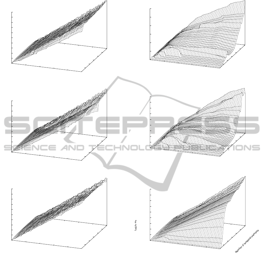
The evaluation of the trigger fact approach is

based on the measurements for the three conﬁgura-

tions shown in Fig. 9. The measurements for all

three conﬁgurations shown in Fig. 9(a), Fig. 9(b),

and Fig. 9(c) lead to the conclusion that this approach

performs pretty good as long as only temporal facts

or temporal rules are used but we see a huge change

to the worse if they are combined.

The temporal nodes approach was evaluated based

on the measurements for the three conﬁgurations

shown in Fig. 10. The measurements for alle three

conﬁgurations shown in Fig. 10(a), Fig. 10(b), and

Fig. 10(c) reﬂect that it performs a little bit better

than the trigger fact approach but as worse in the case

of using temporal facts and rules combined.

5 CONCLUSIONS

AND OUTLOOK

The analysis of the implemented approaches shows

that the current implementation of the RBS Jamocha

can process among 2500 temporal elements per sec-

ond without producing a processing time lag. From

this value we can derive how many temporal elements

can be processed in a rule-based application within

MECHANISMS FOR TEMPORAL LOGIC IMPLEMENTATION IN RULE-BASED SYSTEMS

511

Time in s

Lag in ms

Number of temporal elements

1000

2000

3000

4000

5000

500

1000

1500

2000

2500

3000

3500

4000

4500

5000

(a) Temporal facts

Time in s

Lag in ms

Number of temporal elements

1000

2000

3000

4000

5000

500

1000

1500

2000

2500

3000

3500

4000

4500

5000

(b) Temporal rules

Time in s

Lag in ms

Number of temporal elements

1000

2000

3000

4000

5000

500

1000

1500

2000

2500

3000

3500

4000

4500

5000

Figure 8: Processing lag for temporal facts and rules using

the time fact approach.

the given processing interval of one second. Further-

more, we can derive the expected processing lateness

or system imprecision if a rule-based application re-

quires a higher number of temporal elements than the

estimated value.

However, with the help of this system parame-

ter a rule-based application must be designed in ad-

vanced and the design considerations with respect to

time lags for temporal elements have to remain still

valid, even if the RBS is overloaded. To overcome

this drawback it seems suitable to introduce a special

system fact, similar to the time fact discussed above.

Time in s

Lag in ms

Number of temporal elements

1000

2000

3000

4000

5000

500

1000

1500

2000

2500

3000

(a) Temporal facts

Time in s

Lag in ms

Number of temporal elements

1000

2000

3000

4000

5000

200

400

600

800

1000

1200

1400

1600

1800

(b) Temporal rules

Time in s

1000

2000

3000

4000

5000

500

1000

1500

2000

2500

3000

3500

4000

4500

Figure 9: Processing lag for temporal facts and rules using

the temporal trigger facts approach.

This fact should provide the respective actual time lag

of the RBS and the expected time lag for the next ﬁre

cycle (based on the number of activated and nearly

activated rules). Further investigations will focus on

the prediction of the time lag produced by process-

ing temporal elements in RBS to allow the design of

adaptive rule-based applications with variable or dif-

ferentiated requirements for processing lateness.

ICAART 2011 - 3rd International Conference on Agents and Artificial Intelligence

512

Time in s

Lag in ms

Number of temporal elements

1000

2000

3000

4000

5000

1000

2000

3000

4000

5000

(a) Temporal facts

Time in s

Lag in ms

Number of temporal elements

1000

2000

3000

4000

5000

1000

2000

3000

4000

5000

(b) Temporal rules

Time in s

Lag in ms

Number of temporal elements

1000

2000

3000

4000

5000

1000

2000

3000

4000

5000

Figure 10: Processing lag for temporal facts and rules using

the temporal nodes approach.

REFERENCES

Baader, F., Calvanese, D., McGuinness, D., Nardi, D., and

Patel-Schneider, P., editors (2003). The Description

Logic Handbook. Cambridge University Press.

Forgy, C. L. (1990). Rete: a fast algorithm for the many

pattern/many object pattern match problem. In Expert

systems: a software methodology for modern applica-

tions, pages 324–341, Los Alamitos, CA, USA. IEEE

Computer Society Press.

Hill, E. F. (2003). Jess in Action: Java Rule-Based Systems.

Manning Publications Co., Greenwich, CT, USA.

Krempels, K.-H., Christoph, U., and Wilden, A. (2009).

Jamocha – a Rule-based Programmable Agent. In In-

ternational Conference on Agents and Agent Technol-

ogy 2009 (ICAART’09), INSTICC Setubal, Porto.

Lin, P. and Krempels, K.-H. (2008). A temporal logic

extension for the rete algorithm. Technical report,

Jamocha.org.

Ross, R. G. (2003). Principles of the Business Rules Ap-

proach. Addison Wesley.

MECHANISMS FOR TEMPORAL LOGIC IMPLEMENTATION IN RULE-BASED SYSTEMS

513