PREPROCESSING IN MAGNETIC FIELD IMAGING DATA

Dania Di Pietro Paolo

BMDSys Production, Jena, Germany

Tobias Toennis

Medizinische Abteilung Asklepios Klinik St. Georg, Hamburg, Germany

Sergio Nicola Erne

BMDSys Production, Guenzburg, Germany

Keywords:

Magnetic ﬁeld imaging, Magnetocardiography, Signal preprocessing.

Abstract:

Magnetic Field Imaging (MFI) is a new method of diagnosis of increasing importance in cardiology. MFI

records the magnetic ﬁelds (MF) of the electrical activity of the heart using many extremely sensitive sensors

and displays them afterwards in a clinically applicable manner. Due to the relatively low signal to noise ratio

(SNR) of the magnetic data, the recorded data are often averaged before analysis.

We describe a standardized preprocessing method to be used before averaging MFI data with low SNR. The

reported examples are data from 20 subjects out of a normal cohort examined at the Asklepios Klinik St.

Georg.

1 INTRODUCTION

Magnetic ﬁeld imaging (MFI) is a new non-invasive

method that combines the recording of external mag-

netic ﬁeld (MF) generated by the electrical activity of

the heart with its clinically applicable spatio-temporal

visualization. Cardiac MFs are very weak in compari-

son to the earth magnetic ﬁeld and to electromagnetic

disturbances. To reduce the environment noise, mag-

netic acquisitions are normally carried out in magnet-

ically shielding rooms (MSRs). Unfortunately high

performances MSRs are very expensive and cannot

be easily integrated in the patient logistic of hospitals;

for this reason much effort has been made in order to

develop MFI systems usable in clinical environment.

To achieve this goal it has been necessary to redis-

tribute the task of noise reduction into the three main

components:

• shielding

• design of the sensor system

• data preprocessing

Here, the standardized preprocessing that is used for

collecting data routinely under clinical conditions is

presented.

2 MATERIALS

Twenty subjects (37± 14 years, 6 males, 14 females)

with no history of cardiac diseases have been selected

from a cohort of healthy controls. Written informed

consent has been obtained. The MFI recordings are

carried out at the Asklepios Hospital St. Georg in

Hamburg (Germany) using an Apollo CXS system

(BMDsys Production GmbH, Germany). Apollo CXS

is a 55-channels superconducting quantum interfer-

ence device (SQUID) gradiometer system arranged in

a hexagonal matrix, which covers an area of approxi-

mately 28 cm. The volunteers lie in a supine position

during the recording. The cryostat is placed at ap-

proximately 1 cm distance to the anterior chest wall

above the heart (Figure 1). The MFI sensor system

is operating inside a light magnetically shielded room

(Figure 2).

The data are sampled with a rate of 8200 samples

per second and stored at a sampling rate of 1025 Hz

(the bandwidth is set between 0.016 Hz and 256 Hz).

Recording duration is at least 180s.

463

Di Pietro Paolo D., Toennis T. and Nicola Erne S..

PREPROCESSING IN MAGNETIC FIELD IMAGING DATA.

DOI: 10.5220/0003160504630466

In Proceedings of the International Conference on Bio-inspired Systems and Signal Processing (BIOSIGNALS-2011), pages 463-466

ISBN: 978-989-8425-35-5

 2011 SCITEPRESS (Science and Technology Publications, Lda.)

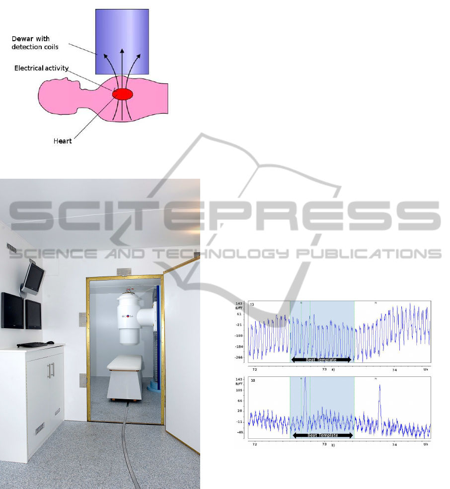
Figure 1: Model of MFI recording.

Figure 2: Biomagnetic system: view from the preparation

room into the acquisition room with patient bed and sensor

system.

3 METHODS

3.1 Real Time Preprocessing

The ﬁrst step to be performed is disturbance subtrac-

tion. To compensate the noise generated by external

interferences, such disturbances are sensed by refer-

ences sensors and a suitable linear combination of

them is calculated for each channel. Then the result

of this operation is subtracted from the recording sen-

sors (Vrba, 1996). Successively, the signals are high

pass ﬁltered using a RC type ﬁlter of the ﬁrst order

with a time constant of 10 s. Before decimation and

low pass ﬁltering, a proprietary adaptive comb ﬁlter

is used to eliminate the power line interference and its

harmonics. The comb ﬁlter introduces no phase shift.

Eventually, the data stream is decimated iteratively in

step of two to obtain the storing rate of 1025Hz. In

each decimation step an anti-aliasing ﬁlter with a rel-

ative cut-off frequency of 0.25 is used.

3.2 Segmentation

To perform averaging, the data stream has to be seg-

mented around each QRS complex. At the beginning

of the off-line analysis the operator iteratively selects

the suitable template parameters (Figure 3). Using the

template, the beats are selected according to the max-

imum coherence matching (MCM) algorithm. Then

the beats list is used as input in the categorized clus-

ter analysis (CCA).

Figure 3: Raw data in two channels: a) The upper panel

shows a channel with a transient vibration picked around

14-15 Hz, b) The lower panel shows a channel with very

high SNR. The beat with blue background is the beat used

for deﬁning the template parameters.

3.3 Categorized Cluster Analysis and

Averaging

A modiﬁed version of CCA is used in order to ﬁnd the

beats to be used in the averaging algorithm. The prob-

lem with the original version of CCA is that in case

the noise is homogeneously distributed over time, the

number of rejected beats can be very high since the

chosen beats are related to only one of the branches

BIOSIGNALS 2011 - International Conference on Bio-inspired Systems and Signal Processing

464

Figure 4: Schematic illustration of a dendrogram which is

the graphical representation of the cluster analysis. Follow-

ing the arrows at each node, the largest group of beats with

the smallest similarity distance is found and thus the start-

ing point for function SNR. The horizontal axis represents

the observations (beats), the vertical axis gives the distance

(or dissimilarity measure).

(Figure 4). For this reason, in order to include more

beats to the average procedure, the distance matrix D,

used in the cluster analysis, is weighted using the av-

erage of the most similar beats in the branch taken

into consideration. At each step the closest beat is

added. In this way a larger number of beats for the

average can be reached when compared to the stan-

dard CCA. Using these beats the averaging procedure

is performed. For further information related to CCA,

please refer to (Di Pietro Paolo et al., 2005).

3.4 Transformation to a Standardized

Sensor Conﬁguration

A localized source

j positioned 15 cm below the sen-

sor 0 (center of the sensor system) is used for con-

version based on multipole expansion (ME). Param-

eters till octupole, as proposed by Burghoff et all,

(Burghoff et al., 2000) are used in Cartesian space.

Using these terms, it is possible to reconstruct a 55-

channel averaged signal. A ME is a series expansion

that can be used to represent the ﬁeld produced by

a source (in this case heart) in terms of expansion pa-

rameters which become small as the distance from the

source increases. Katila and Karp (Katila and Karp,

1983) proved the possibility to describe the heart sig-

nal by expansion of the magnetic multipoles up to the

octupole term. It is interesting to note that the mag-

netic dipolar term serves as a good approximation in

the early ventricular activation (Trontelj et al., 1991).

By adding more terms (quadrupoles and octupole) a

very accurate reconstruction of the sources can be ob-

tained. The magnetic multipole expansion as the fol-

lowing form:

B(~r) = −

4π

∞

∑

n=0

∞

∑

m=0

∇



n+1

(cosθ)e

−imζ



(1)

n+ 1

∇

′



cosθ

′



imζ

′

x,~r

′



′



′

Here are γ

the coefﬁcients so that (Katila and Karp,

1983):

= [2− δ(m)]

(n− m)!

(n+ m)!

with P

(cosθ) the associated Legendre functions of

ﬁrst kind. The current density

j in the expression 1

is the total current density over the volume v

′

and the

expansion is valid for the region lying outside the sur-

face S

′

, i.e. r should exceed the largest value of r

′

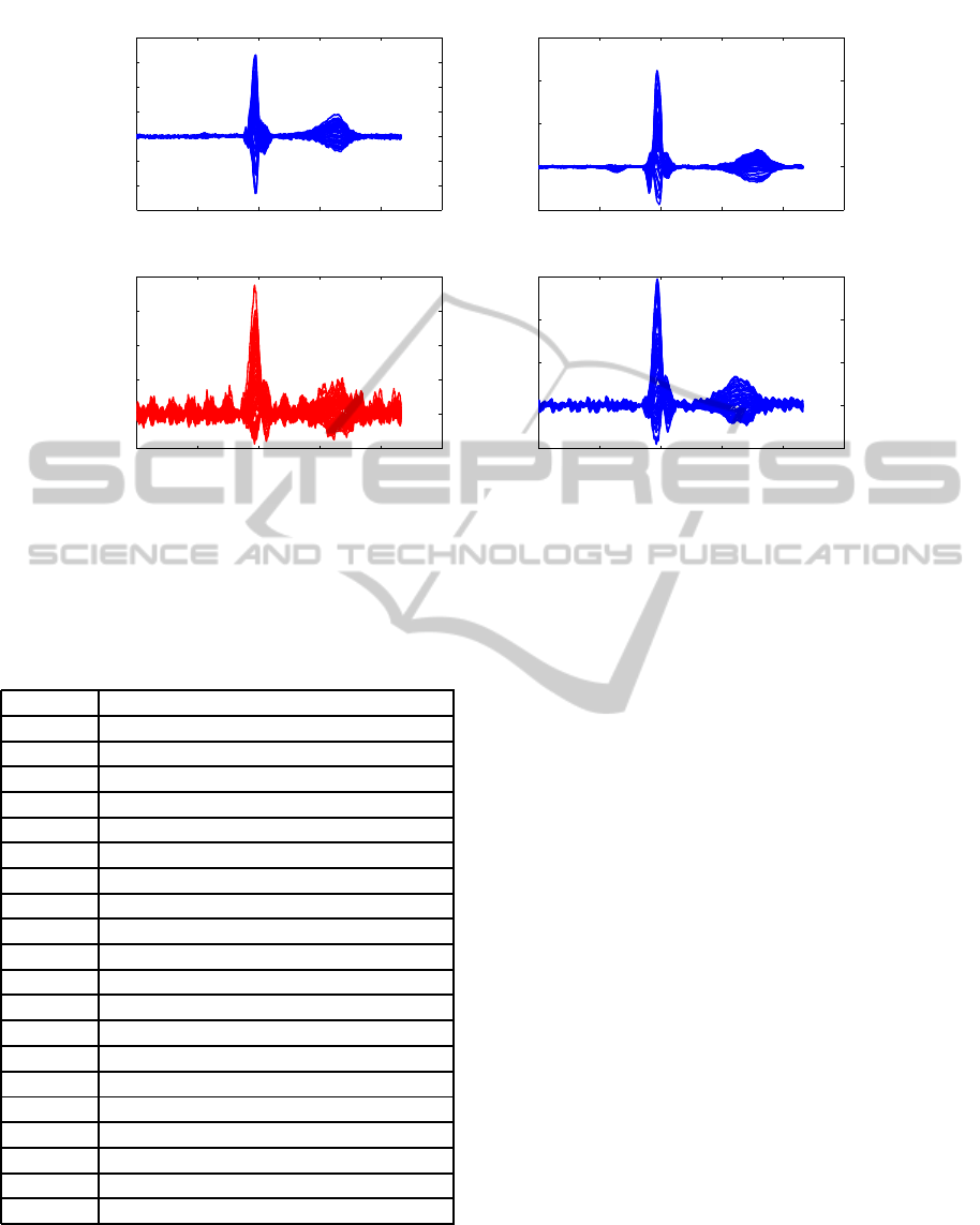
4 RESULTS

The preprocessing is applied to the 20 acquisitions.

The performances of the preprocessing in terms of

noise reduction are measured using the Root Mean

Square (RMS) before and after the application of

CCA and transformation to a standard sensor con-

ﬁguration. The SNR has been applied on the av-

eraged magnetic signals in the segment [T-end, P-

onset], since in this region the signal amplitude is usu-

ally very low. A summary of the results is shown in

table 1. The application of CCA and ME improved

the SNR of the averaged magnetic signals in almost

all cases up to 90%. Only in one case the preprocess-

ing was not successful. Examples of averaged signals

are shown in Figure 5.

5 DISCUSSION AND

CONCLUSIONS

The preprocessing of MFI data outlined here is the

basis for all speciﬁc analysis that can be performed

with the MFI software of Apollo CXS (QRS frag-

mentation analysis, digital subtraction MFI for stress

induced ischemia detection etc). It has been shown

that combining a carefully designed low cost shielded

room (patent DE 10 2007 017 316 B4) with a gra-

diometric sensor system it is possible to obtain data

usable in clinical environment. Furthermore, the use

of a dedicated algorithm for the averaging procedure

PREPROCESSING IN MAGNETIC FIELD IMAGING DATA

465

0 200 400 600 800 t/ms

−6

−4

−2

x 10

B/fT

0 200 400 600 800 t/ms

−5

x 10

B/fT

0 200 400 600 800 t/ms

−5

x 10

B/fT

0 200 400 600 800 t/ms

−5

x 10

B/fT

Figure 5: Averaged magnetic signals using Apollo CXS: a), b) averaged magnetic signals after CCA and transformation to

standard sensor conﬁguration (Subject 6 and 7, respectively); Subject 10 before (red) c) and after d) (blue) application of CCA

and ME.

Table 1: Noise reduction percentage in the 20 subjects after

applying CCA and standard sensor conﬁguration transfor-

mation

Subjects Noise Reduction (%) after CCA + ME

1 33,76%

2 61,44%

3 65,05%

4 53,62%

5 -43,00%

6 74,52%

7 60,08%

8 35,49%

9 64,87%

10 68,29%

11 91,99%

12 62,83%

13 15,39%

14 56,98%

15 33,27%

16 14,14%

17 91,48%

18 16,73%

19 40,14%

20 91,28%

and the transformation to standard sensor conﬁgura-

tion make it possible to obtain data of quality com-

parable to those obtained in much more complicated

and expensive systems.

REFERENCES

Burghoff, M., Nenonen, J., Trahms, L., and Katila, T.

(2000). Conversion of magnetocardiographic record-

ings between two different multichannel squid de-

vices. Trans. Biol. Eng., 47(7):869–875.

Di Pietro Paolo, D., M¨uller, H.-P., and Erne, S. N. (2005).

A novel approach for the averaging of magnetocar-

diographically recorded heart beats. Phys Med Biol,

50(10):2415–2426.

Katila, T. and Karp, P. (1983). Magnetocardiography: Mor-

phology and multipole presentations. In Biomag-

netism: An interdisciplinary approach, pages 237–63.

S J. Williamson, G L. Romani, L Kaufman, I Modena.

Plenum Press, New York.

Trontelj, Z., Jazbinsek, V., Erne, S., and Trahms, L. (1991).

Multipole expansions in the representation of current

sources. Acta Oto-laryngologica, 111:88–93.

Vrba, J. (1996). SQUID gradiometers in real environments.

In Weinstock, H., editor, SQUID Sensors: Funda-

mentals, Fabrication and Application, pages 117–178.

Kluwer Academic Publishers.

BIOSIGNALS 2011 - International Conference on Bio-inspired Systems and Signal Processing

466