A HIERARCHICAL VENDOR SELECTION OPTIMIZATION

TECHNIQUE FOR MULTIPLE SOURCING

Mariagrazia Dotoli

Dipartimento di Elettrotecnica ed Elettronica, Politecnico di Bari, Via Re David 200, 7015 Bari, Italy

Marco Falagario

Dipartimento di Ingegneria Meccanica e Gestionale, Politecnico di Bari, Via Re David 200, 7015 Bari, Italy

Keywords: Business Intelligence, Supply Chain Management, Supplier Evaluation and Selection, Decision Support

System, Data Envelopment Analysis, Analytic Hierarchy Process, Linear Programming.

Abstract: The paper addresses a crucial objective of the strategic function of purchasing in supply chains, i.e., vendor

rating, proposing a hierarchical model for supplier business intelligence. A three-level optimization process

for supplier selection in a multiple sourcing strategy context is proposed. First, the Data Envelopment

Analysis, the most widespread method for supplier selection, is used to evaluate the efficiency of suppliers.

Second, the well-known Analytic Hierarchy Process is applied to rank the efficient suppliers given by the

previous step. Third, a linear programming problem is solved to find the quantities to order from each

efficient supplier. We show the model effectiveness on a simulated case study of a C class component.

1 INTRODUCTION

A Supply Chain (SC) is a business network

interconnecting independent manufacturing and

logistics companies that perform critical functions in

the order fulfilment process (Dotoli et al., 2006).

The SC configuration is essential to pursue a

competitive advantage and meet the market demand.

This paper focuses on one of the strategic

purchasing function tasks in a private SC, i.e.,

vendor ranking (Costantino et al., 2009). Vendor

rating systems identify top suppliers, i.e., the

candidate partners that are best equipped to meet the

customer’s expected level of performance, and

check them periodically. Therefore, vendor selection

is a multi-objective decision problem, including

conflicting objectives such as, besides the obvious

goal of (low) price, quality, quantity, delivery,

performance, capacity, communication, service,

geographical location etc. (Degraeve et al., 2000).

Numerous multi-criteria decision making

approaches have been suggested to solve the vendor

evaluation and selection problem and, among these,

individual approaches and integrated ones can be

distinguished. The most important individual

methods are: the Data Envelopment Analysis

(DEA), mathematical programming, the Analytic

Hierarchy Process (AHP), case-based reasoning,

fuzzy decision making, genetic algorithms and many

more. The so-called integrated approaches join

together different techniques (e.g., integrated AHP,

DEA, and artificial neural networks, integrated AHP

and goal programming, etc.). Individual approaches

are more popular than integrated ones, with the most

widespread individual technique being DEA, due to

its robustness (Ho et al. 2010) and its ability to be

implemented also considering qualitative criteria: as

an example, Talluri et al. (2006) extend the classical

DEA technique considering risk evaluation.

However, DEA presents the drawback that its

efficient alternatives are by definition equally

optimal and no difference can be singled out with

respect to their different effectiveness.

In the private sector, the buyer can choose

between a single or multiple sourcing approach.

Single sourcing is defined as the fulfilment of all

corporate requirements for a particular product by a

selected supplier. On the other hand, multiple

sourcing is the splitting of an order among multiple

sellers, i.e., the company has two (dual sourcing) or

195

Dotoli M. and Falagario M..

A HIERARCHICAL VENDOR SELECTION OPTIMIZATION TECHNIQUE FOR MULTIPLE SOURCING.

DOI: 10.5220/0003088801950200

In Proceedings of the International Conference on Knowledge Management and Information Sharing (KMIS-2010), pages 195-200

ISBN: 978-989-8425-30-0

 2010 SCITEPRESS (Science and Technology Publications, Lda.)

more suppliers for the same component. Obviously,

each solution presents advantages and drawbacks.

In this paper we propose a hierarchical strategy

for optimal supplier evaluation and selection in

multiple sourcing supplies based on three levels.

First, we use the well-known DEA method to

evaluate the weights of input and output criteria and

divide suppliers into two categories: efficient and

inefficient ones. Second, we apply the widespread

decision making AHP technique (Saaty, 1990) to

rank the efficient alternatives and select the effective

ones. AHP is a multi-objective decision technique in

which all the elements of the decision problem

(overall goal, criteria, alternatives) are arranged in a

hierarchical structure and objectives are of varying

degrees of importance. Although in many cases

optimization methods lead to similar results, here we

select AHP because it relies on pairwise

comparisons of the solutions, providing an approach

to rank alternatives based on their reciprocal

assessment. Third, after ranking the efficient

solutions and identifying the most effective ones, a

linear programming problem is solved to calculate

the quantities of product to require from each

effective supplier in the multiple sourcing context.

Summing up, we provide a decision support tool for

supplier business intelligence, to rank vendors and

provide the buyer with a simple instrument to

determine the quantities to order from each effective

supplier in a multiple sourcing strategy context.

2 THE HIERARCHICAL

SUPPLIER SELECTION

TECHNIQUE

A vendor selection problem is defined by a set of

bidding suppliers

{}

, ,.....,

Sss s= and a set of

conflicting criteria

{}

, ,.....,

Ccc c= , according to

which vendors have to be ranked. The criterion set is

partitioned as

CC C=∪, with

{}

, ,.....,

Ccc c= ,

{}

, ,.....,

OHH HK

Ccc c

++ +

= ,

and H+K=n respectively representing the input and

output criteria sets, and the criteria number.

The input criteria are defined as the supplier

attributes considered before the supply takes place

(e.g., price, geographical distance of the supplier,

ICT integration, etc.) while the output criteria are

connected to the supplier once the goods arrive at

the firm (e.g., quality, reliability, lead time, etc.).

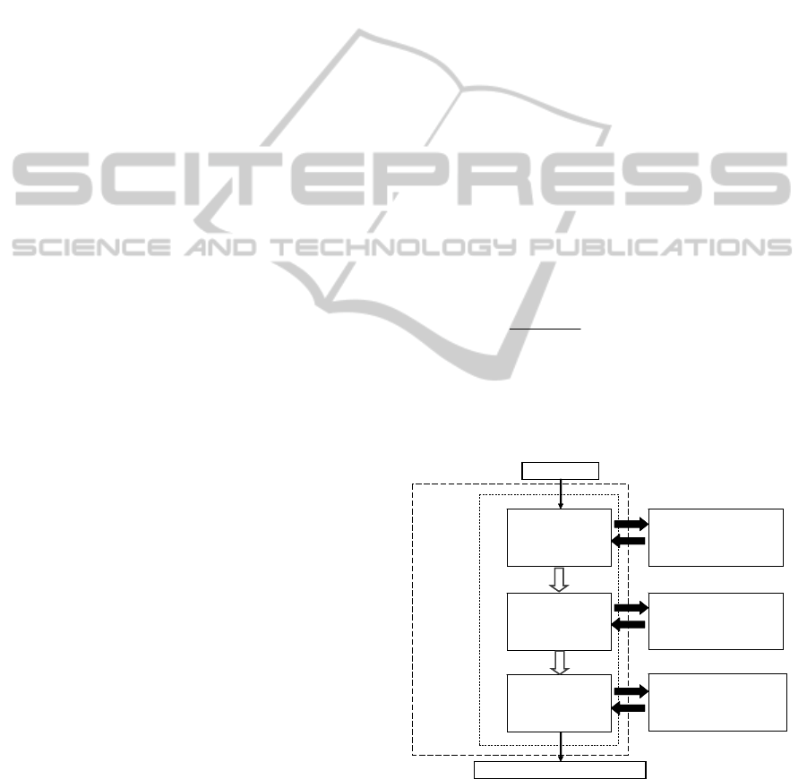
Figure 1 shows the presented hierarchical integrated

approach to determine effective suppliers and the

requested product quantities.

2.1 The First Level of the Hierarchical

Optimization - the DEA Method

The first level of the supplier selection approach in

Fig. 1 employs the Data Envelopment Analysis

(DEA) (Charnes et al., 1978), a linear programming-

based technique for determining the efficiency of

different decision making units. As regards the

application of DEA to supplier selection, the

strength of this technique is the distinction between

input and output performance measures. Input

performance is given by the amount of resource used

by the vendor to carry out the supply process (for

instance, the purchasing price), while output

parameters express how good is the service provided

by the suppliers to the buyer (examples for these are

the quality of purchased product or the timeliness of

deliveries).

The efficiency of supplier

S∈ is defined as:

kkf

hhf

⋅

∑

with f=1,…,F,

(1)

where

) is the k-th (h-th) output (input)

performance for the f-th actor and u

) its weight.

Level 3

Query Linear Programming

Problem solution

Level 2

Query AHP

Level 1

Query DEA

Input Data

(input and output

performance values)

Input Data

for efficient suppliers

(input and output

performance values)

Input Data

for effective suppliers

(PI

i_AHP

AHP

performance values)

Hierarchical

Model

Design

Effectivesuppliers and required quantities

Efficient

suppliers

Ranking of

efficient

suppliers

Required

quantities

from

effective

suppliers

Suppliers set

Level 3

Query Linear Programming

Problem solution

Level 2

Query AHP

Level 1

Query DEA

Input Data

(input and output

performance values)

Input Data

for efficient suppliers

(input and output

performance values)

Input Data

for effective suppliers

(PI

i_AHP

AHP

performance values)

Hierarchical

Model

Design

Effectivesuppliers and required quantities

Efficient

suppliers

Ranking of

efficient

suppliers

Required

quantities

from

effective

suppliers

Suppliers set

Figure 1: The hierarchical supplier selection approach.

In the DEA method, the efficiency of each actor is

obtained by determining the set of coefficients u

and

which maximizes this value, taking into

account that for each actor it holds by definition

KMIS 2010 - International Conference on Knowledge Management and Information Sharing

196

E ≤ . Hence, the measure of supplier efficiency

can be obtained by solving the following

optimization problem for each considered vendor:

max

E with f=1,…,F,

(2)

subject to (s.t.):

kkj

hhj

⋅

≤

⋅

∑

with j=1,…,F,

(3)

uv≥ for k=1,…,K and h=1,…,H.

(4)

Problem (2)-(3)-(4) can be linearized by

minimizing the inputs and keeping fixed output

values (input-oriented method) or maximizing the

outputs and keeping fixed input values (output-

oriented method) (Wang and Chin, 2010). Using the

latter solution, the problem is modified as follows:

max

fkkf

Euy

=⋅

∑

with f=1,…,F,

(5)

s.t.:

kkj hhj

uy vx

⋅− ⋅≤

∑∑

with j=1,…,F,

(6)

hhf

⋅=

∑

with f=1,…,F,

(7)

and (4).

The efficiency of analyzed suppliers can be found

solving problem (5)-(6)-(7)-(4) for each

f-th supplier

for

f=1,2 ,…,F. Obviously, the f-th vendor is

maximally efficient if

=1. Therefore, suppliers can

be ranked based on their efficiency value

2.2 The Second Level of the

Hierarchical Optimization - the

AHP Approach

The Analytic Hierarchy Process (AHP) is a multi-

objective decision technique (Saaty, 1990) for

ranking a number of alternatives according to a set

of conflicting criteria of various degrees of

importance. This paper selects AHP to single out in

the second level of the optimization the effective

suppliers among efficient ones determined at the

first level since, being based on alternatives pairwise

comparison, AHP turns out to exhibit an enhanced

accuracy with respect to other decision making

techniques. AHP consists of the following steps.

Step 1. Structuring the decision problem as a

hierarchy.

Select the first level of the hierarchical

structure as the overall goal “Effectiveness”. Define

the second level, composed by the

n criteria

contributing to the goal. Determine the third level as

the

m alternative suppliers to be ranked in terms of

the criteria in the second level.

Step 2. Constructing the decision matrix.

Determine the decision matrix D of dimensions mxn,

where m is the number of alternatives (the efficient

suppliers),

n is the number of criteria, and element

with i=1,…,m and j=1,…,n measures the i-th

supplier performance against criterion c

Step 3. Constructing the pairwise comparison

matrix

. Compare the n criteria with each other

and construct the nxn pairwise comparison matrix

by Saaty’s original AHP scale in Table 1. More

precisely, determine each element

c of C

with

i,j=1,…,n, representing the relative importance of

the i-th criterion compared to the j-th one, by

interviewing the buyer evaluating the importance of

criterion

over c

and associating it an integer value

from 1 to 9 according to Table 1. Obviously, less

important criteria are defined by reciprocals

= for each i,j=1,…,n.

Step 4. Determining the eigenvector associated

to the maximum eigenvalue of the comparison

matrix

. Calculate the eigenvalues set

{

,…,

} of C

, where R is its rank. Let

max

be the maximum eigenvalue of C

, then determine

its eigenvector v

max

. Compute the priority vector:

[...]

npp=⋅=

max

(8)

where each element p

with j=1,…,n of P represents

the importance degree of the j-th performance index

associated to the j-th column of D’: the greater p

the more important the j-th performance index.

Step 5. Raising alternatives to the criteria power.

Determine the alternative values associated to each

j-th performance index as follows:

[ ... ]

CRIT .

(9)

A HIERARCHICAL VENDOR SELECTION OPTIMIZATION TECHNIQUE FOR MULTIPLE SOURCING

197

Table 1: Saaty’s AHP scale of comparisons.

Intensity of importance Definition

1 Equal importance

3 Moderate importance

5 Strong importance

7 Very strong importance

9 Extreme importance

2,4,6,8 Intermediate values between

the two adjacent judgments

for each j=1,…,n. Determine the following vectors.

=[g

… g

[...]

jjj

ppp

jmj

dd=

CRIT .

(10)

for each j=1,…,n.

Step 6. Determining the decision model. For each

alternative i with i=1,…,m, determine:

(

)

min ,...,

iAHP i in

PI g g=

(11)

so that PI

i_AHP

provides information about the

satisfaction of alternative s

with respect to the

performance indices and their importance degree.

Step 7. Ranking the alternatives. Suppliers are

ranked according to index PI

i_AHP

: the best supplier

is the one showing the highest index PI

i_AHP

2.3 The Third Level of the Hierarchical

Optimization: the Linear

Programming Methodology

Linear programming is a mathematical optimization

process in which a single objective function states

mathematically what is being maximised, e.g.,

profit, or minimized, e.g., cost.

With the aim of determining the quantities to

require from the most effective suppliers singled out

in the previous and second level of the hierarchical

supplier evaluation procedure, we define the Supply

Evaluation Index (SEI) as follows:

iiAHP

SEI q PI

=⋅

∑

(12)

that is an overall index measuring the efficiency on

the supply considering the μ≤m most effective

suppliers obtained by the second-level AHP

optimization among the m efficient vendors obtained

by the first-level DEA optimization. In particular,

variables q

with i=1,.., μ are the percentage

quantities of product with values ranging from 0 to 1

to request from each vendor to obtain the supply.

Hence, the linear programming problem is:

()

ax SEI

(13)

s.t.:

∑

(14)

≤

with 01

≤

≤ and i=1,…, μ,

(15)

≥ with

≤

∑

(16)

In particular, δ

is a parameter measuring the

minimum percentage quantity (eventually equal to

zero) that the buyer decides to buy from each

effective supplier independently from its ranking to

keep the long-term partnership. In addition, γ

is the

given production capacity (expressed in percentage

values in a 0-1 range) of the i-th effective supplier

with i=1,…,μ. Hence, (14) guarantees that the whole

requested quantity is supplied, constraints (15) are

connected to the quantities each supplier is able to

deliver, (16) models the buyer will of requiring

products from each efficient supplier independently

from the ranked position.

3 THE CASE STUDY

To show the effectiveness of the presented

hierarchical approach, we consider a simulated case

study requiring the supply of C class components

under multiple sourcing and assuming that the

number of existing suppliers equals F=15. We

remind that spare parts in inventory are usually

divided in the literature into three classes according

to their money usage (Krajewski and Ritzman,

2002): class A items typically represent only about

20% of the items but account for 80% of the money

usage; class B components account for additional

30% of the items but only for 15% of the money

usage; finally, 50% of the items falls in class C,

representing a mere 5% of financial usage. While for

A and B components a strategic partnership between

buyer and seller is typically created (so that often

single sourcing is applied), C components are such

that an increasing competition among suppliers

usually allows the buyer to obtain a better price:

hence, it is important to rank suppliers and decide

the quantities to request them by different criteria.

The case study vendor efficiency is estimated

using H=2 input criteria, namely:

KMIS 2010 - International Conference on Knowledge Management and Information Sharing

198

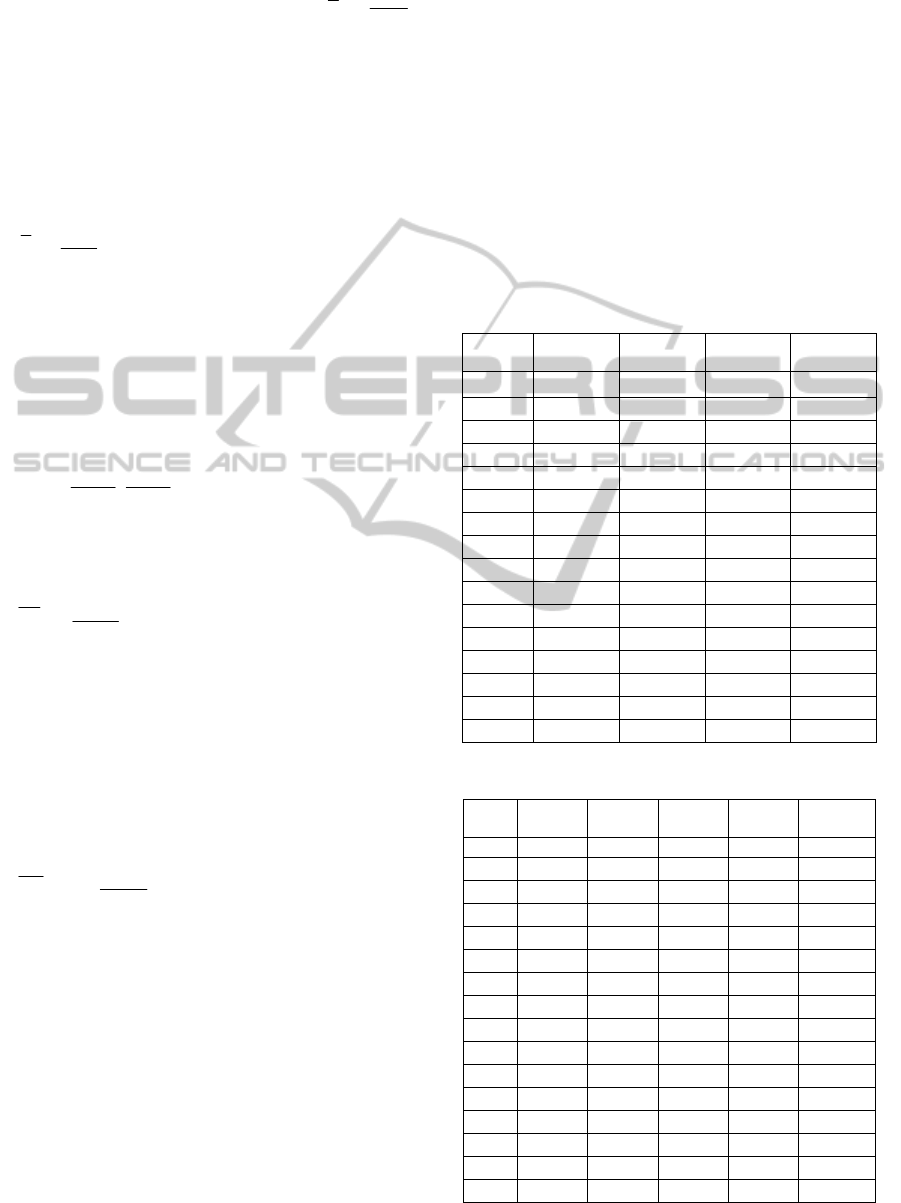
 price - This attribute measures the price offered

by each supplier. It is evaluated as

max

with f=1,…,F, where p

is the offered price and

max

1,2,...,

max ( )

= the maximum offered price;

 geographical distance - this criterion expresses

the geographical distance of the supplier from

the buyer. The nearer the supplier, the lower the

transportation costs. The normalized

performance of the f-th supplier with f=1,…,F is

max

, where d

is the vendor distance and

max

1,2,...,F

max ( )

the maximum distance.

The K=2 considered output criteria are:

 quality - this criterion is strictly related to the

number of accepted products: indeed, a high

number of defects means high costs of

restoration. Hence, we define the index quality of

the f-th supplier with f=1,…,F as

af af

vf vf

pc lot

=⋅

, where pc

a,f

(pc

v,f

) is the

number of accepted (verified) items and lot

a,f

(lot

v,f

) is the amount of accepted (verified) lots.

The normalized quality index is hence

max

, with

max

1,2,...,F

max ( )

QIQ

;

 lead time - This criterion is related to the supplier

manufacturing capability and flexibility. The

lead time is defined as the time span between the

placing of an order and the receipt of goods.

Obviously, the shorter the lead time, the better

the supplier in term of flexibility, production

capability and internal organization. Given the

lead time index LT

of the f-th supplier with

f=1,…,F, the normalized lead time is

max

=−

, with

max

1,2,...,

max ( )

LT LT

The normalized input performance values of each

supplier are collected in Table 2 (second and third

column). In the second-last and last column of Table

2 the output indices are reported.

Applying the DEA approach, problem (5)-(6)-

(7)-(4) is defined and solved, so that the results in

Table 3 are obtained. Analysing Table 3, the

efficient suppliers are supplier 3, 5, 10, 11, and 14,

so that m=5 suppliers are singled out. For example,

supplier 3 is efficient by weighting the price

criterion u

=0.389, the normalized geographical

distance u

=3.591, the quality index v

=0.517, and

the lead time index v

=0.942.

The next step is to rank the efficient suppliers 3,

5, 10, 11, and 14 in order to calculate the quantities

to require for a supply. The results of the AHP

optimization are shown in Table 4, collecting the

performance values of vendors s

with

f=3,5,10,11,14. The second column reports

performance index PI

i_AHP

and the last column ranks

the five efficient suppliers: the best supplier is s

showing a high value of lead time and a low value of

price (the lowest), together with an intermediate

geographical distance and a high quality index.

Following are suppliers s

, s

, and s

Table 2: The data for the DEA input and output criteria.

Supplie

Input 1 Input 2 Output 1 Output 2

0.689 0.456 0.894 0.237

1.000 0.538 0.998 0.347

0.798 0.192 0.985 0.521

0.790 0.594 0.946 0.125

0.589 0.066 0.902 0.000

0.487 0.987 0.945 0.568

0.897 1.000 0.976 0.625

0.657 0.456 0.928 0.544

0.984 0.732 1.000 0.875

0.123 0.450 0.756 0.757

0.235 0.200 0.912 0.359

0.357 0.759 1.000 0.915

0.573 0.417 0.350 0.830

0.233 0.350 0.870 0.765

0.467 0.897 0.910 0.935

Table 3: The first-level DEA optimization data and results.

Supplie

Weight Weight Weight Weight Efficiency

f u

0.520 1.407 0.443 0.000 0.396

0.168 1.547 0.223 0.406 0.363

0.389 3.591 0.517 0.942 1.000

0.417 1.129 0.355 0.000 0.336

1.303 3.525 1.109 0.000 1.000

1.358 0.343 0.425 0.000 0.402

0.122 0.890 0.094 0.338 0.303

0.251 1.831 0.193 0.695 0.557

0.090 1.245 0.000 0.597 0.522

1.695 1.759 0.000 1.321 1.000

2.442 2.131 0.949 0.374 1.000

1.095 0.802 0.330 0.325 0.628

0.158 2.181 0.000 1.046 0.868

1.463 1.883 0.499 0.740 1.000

0.715 0.742 0.000 0.558 0.521

A HIERARCHICAL VENDOR SELECTION OPTIMIZATION TECHNIQUE FOR MULTIPLE SOURCING

199

Table 4: The second-level AHP optimization results.

Efficient supplierPerf. index Position

iAH

0.132 4

0.117 5

0.273 1

0.219 3

0.258 2

Table 5: The third-level linear programming problem data.

Supplier Minimum requested quantity Capacity

f δ

10 0.200 0.600

11 0.200 0.400

14 0.200 0.700

Table 6: The third-level linear programming results.

Supplier Required quantity

f q

10 0.400

11 0.200

14 0.400

After rnking the efficient suppliers, the linear

programming problem (13)-(14)-(15)-(16) is defined

and solved for a multiple sourcing strategy with μ=3.

The values of minimum required quantities δ

and

percentage capacities γ

of suppliers are collected in

Table 5. Table 6 shows the results of the linear

programming problem solution, i.e., the required

quantities from the three effective suppliers s

, s

and s

. Results show that 40% of the supply will be

provided in turn by each of the two most effective

suppliers, i.e., s

and s

, whereas the remaining

20% of the requested product will be provided by

the third-ranked supplier s

4 CONCLUSIONS

The paper focuses on a crucial issue of purchasing in

supply chains, i.e., vendor evaluation and selection.

A novel three-step methodology based on the Data

Envelopment Analysis (DEA) approach, the

Analytic Hierarchy Process (AHP), and linear

programming is presented. At the first level of the

hierarchical technique, a vendor rating technique

based on DEA is devised to obtain efficient and

inefficient suppliers. Hence, the AHP process is

applied to rank the efficient vendors based on the

overall performance index. Finally, a linear

programming problem is solved to split the supply

adopting a multiple sourcing strategy. To the best of

the authors’ knowledge, no one in the related

literature has ever joined these three approaches for

supplier selection in such a context. A numerical

case study shows the effectiveness of the presented

three step method for a C class component. Future

perspectives are identifying a real case study to

further verify the approach flexibility and simplicity

of use by the firm purchasing manager.

ACKNOWLEDGEMENTS

This work was supported by the TRASFORMA

“Reti di Laboratori” network funded by Apulia

Italian Region.

REFERENCES

Charnes A., Cooper W.W., Rhodes E., 1978. Measuring

the efficiency of decision making units; European

Journal of Operational Research, 2, 429–444.

Costantino N., Dotoli M., Falagario M., Fanti M.P.,

Iacobellis G., 2009. A Decision Support System

Framework for Purchasing Management in Supply

Chains, Journal of Business and Industrial Marketing,

24(3/4): 278-290.

Degraeve Z., Labro E., Roodhooft F., 2000. An evaluation

of vendor selection models from a total cost of

ownership perspective; European J. of Operational

Research, 125(1), 34-58.

Dotoli M., Fanti M.P., Meloni C., Zhou M.C., 2006.

Design and optimization of integrated e-supply chain

for agile and environmentally conscious

manufacturing, IEEE Transactions on Systems Man

and Cybernetics, part A, 36(1), 62-75.

Ho W., Xu X., Dey P.K., 2010. Multi-criteria decision

making approaches for supplier evaluation and

selection: A literature review, European Journal of

Operational Research, 202, 16-24.

Krajewski L., Ritzman L., 2002. Operation Management:

Strategy and Analysis, Prentice Hall, London, UK, 6th

ed.

Saaty T.L., 1990. How to Make a Decision: the Analytic

Hierarchy Process, European Journal of Operational

Research, 48:9-26.

Talluri, S., Narasimhan, R., Nair, A., 2006. Vendor

performance with supply risk: A chance-constrained

DEA approach; International Journal of Production

Economics 100(2), 212–222.

Wang Y.-M., Chin K.-S., 2010. A neutral DEA model for

cross-efficiency evaluation and its extension; Expert

Systems with Applications, Elsevier, 37, 3666-3675.

KMIS 2010 - International Conference on Knowledge Management and Information Sharing

200