Application of Self-organizing Maps in Functional
Magnetic Resonance Imaging
Anderson Campelo
1
, Valcir Farias
1
, Marcus Rocha
1
, Heliton Tavares
1
and Antonio Pereira
2
1
Programa de P´os-Graduac¸˜ao em Matem´atica e Estat´ıstica
Universidade Federal do Par´a, Bel´em, Brazil
2
Univesidade Federal do Rio Grande do Norte, Natal, Brazil
Abstract. In the present work, we used Kohonen’s self-organizing map algo-
rithm (SOM) to analyze functional magnetic resonance imaging (fMRI) data. As
a first step to increase computational efficiency in data handling by the SOM al-
gorithm, we performed an entropy analysis on the input dataset. The resulting
map allowed us to define the pattern of active voxels correlated with auditory
stimulation in the data matrix. The validity of the algorithm was tested using both
real and simulated data.
1 Introduction
Functional magnetic resonance imaging (fMRI) is a non-invasive tool widely used for
studying the human brain in action. The fMRI has been applied to cognitive studies
and also in a clinical setting to monitor tumour growth, pre-surgical mapping, and
to diagnose epilepsy, Alzheimer’s disease, etc [1]. The fMRI measurements are based
on blood-oxygen-level-dependent correlations (BOLD) [2],[3], with hemoglobin being
used as endogenous contrast agent, due to the magnetic properties of oxy-hemoglobin
(diamagnetic) and deoxy-hemoglobin (paramagnetic) [4].
The BOLD signal was obtained using two experimental paradigms. The first used a
blocked design, with the subject being exposed to alternating periods of stimulation and
rest. The event-related paradigm, on the other hand, required that the subject performs
a simple task, intercalated by long resting intervals.
A fMRI dataset consists of images in 3D space (x × y × z), with each image point,
named a voxel, changing a long time (t). Most fMRI analysis try to identify how signal
related to voxels in a region of interest (ROI) vary in time and to find out whether
these variations are somehow correlated with the stimulus. This analysis, however, is a
computational challenge due to the low signal to noise ratio in the BOLD response and
the usually large amount of data that needs to be processed. Many analytical methods
have been developed to deal with this complexity, some of them were created earlier to
analyze positron emission topography-generated signals (PET).
Most methods available in the literature use statistical techniques to identify active
regions, including Student’s t test [5], crossed correlation [6], and the general linear
Campelo A., Farias V., Rocha M., Tavares H. and Pereira A. (2010).
Application of Self-organizing Maps in Functional Magnetic Resonance Imaging.
In Proceedings of the 6th International Workshop on Artificial Neural Networks and Intelligent Information Processing, pages 72-80
Copyright
c
 SciTePress

model (GLM) [7]. These methods are based on the standard hemodynamic function,
which models the BOLD response in the brain. Other popular methods are independent
component analysis (ICA) [8], [9] and principal component analysis (PCA) [10].
Clustering techniques have also been used successfully, including K-means, fuzzy
cluster and hierarchical clustering. Clustering techniques are based on the similarity
observed in voxel’s time series. The present study uses the Kohonen’s self-organizing
maps algorithm (SOM) to analyse fMRI data. The SOM [11] is a type of clustering tech-
nique which transforms a signal input pattern of an arbitrary dimension into a discrete
map and implements transformations in a topologically organized way.
2 Material and Methods
2.1 Simulated Data
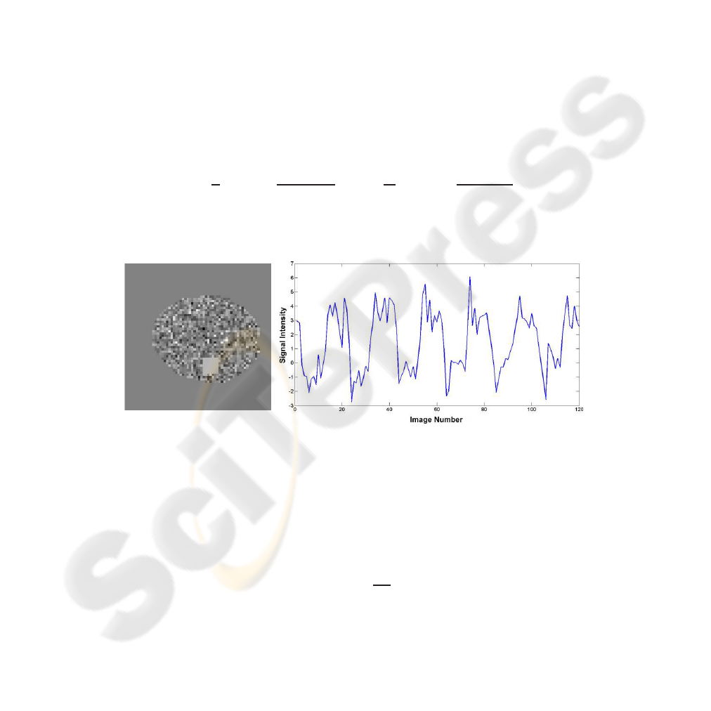
We simulated the fMRI experiment (64 × 64) depicted in Figure 1 with 120 slices by
convoluting a block-like stimulus function with the canonical hemodynamic response
function generated as a sum of two distribution functions [12]:
h(t) =
t
d
!
a
exp
−(t − d
1
)
b
!
− c
t
d
′
!
a
′
exp
−(t − d
′
)
b
′
!
, (1)
with a = 6, a
′
= 12, b = b
′
= 0.9 and c = 0.35, having been determined experimen-
tally by Glover in 1999 with auditory stimulation [13].
Fig.1. Diagram showing the spatial distribution of active voxels and their intensity along time in
simulated data.
The active area corresponds to 49 voxels, while 1349 voxels corresponded to the
remaining grey matter. The other 2698 voxels corresponded to the background and are
not time modulated. We added uniform Gaussian noise to reach a SNR of 2dB, which
was calculated with the following expression:
SNR = 10 log
σ
2
S
σ
2
R
!
, (2)
where σ
2
S
2 and σ
2
R
are signal and noise variances, respectively.

2.2 Real Data
The fMRI experiment used a 1.5 T Siemens scanner (Magnetom Vision, Erlangen, Ger-
many), with the following parameters for EPI (echo-planar imaging) sequences: TE =
60 ms, TR = 4.6 s, FA = 90, FOV = 220 mm, and slice thickness of 6.25 mm. 64 cerebral
volumes with 16 slices each were acquired with a matrix dimension of 128 × 1 28.
During the experimental procedure the subject received auditory stimulation in a
blocked design, with 5 stimulation blocks (27.5s each) intercalated with 6 resting blocks
(27.5 s each). During the task, the subject listened passively to a complex story with a
standard narrative structure. After, the test the subject had to inform to the experimenter
its comprehension of the story content.
Acquired images were preprocessed with the software SPM8 (Statistical Parametric
Mapping) in order to increase the signal-to-noise ratio (SNR) and to eliminate incident
noise associated with the hardware, involuntary movements of the head, cardiac and
respiratory rhythms, etc.
2.3 Self-organizing Maps
fMRI data was analyzed with Kohonen’s SOMs using an implementation available in
the literature (see [14], [15], [16], [17], [18], [19]). Kohonen’s SOM is an artificial
neural network where neurons are disposed as a uni- or bi-dimensional grid layout. In a
bi-dimensional layout, geometriy is free and can be rectangular, hexagonal, triangular
etc. In a SOM, each neuron in a grid is represented by a probability distribution function
of the input data.
The SOM algorithm responsible for map formation begins initializing the grid neu-
rons weights with random values, which can be obtained from the input data. In the
present work we used a bidimensional grid of dimension 10 × 10 (i = 100) [19]. Each
neuron in the grid is connected to every element of the input dataset, i.e., the dimension
of weights m
i
is the same as the input dataset:
m
i
= [m
i1
, m
i2
, . . . , m
in
]
T
∈ ℜ, (3)
where n indicates the total amount of points available in the time series generated by
the fMRI experiment.
After each iteration t of the ANN, we selected randomly a vector from the input
dataset, given by:
x
i
= [x
1
, x
2
, . . . , x
n
]
T
∈ ℜ, (4)
which indicates the time series of a given voxel from the fMRI dataset.
Then, x is compared to weights m
i
in the grid using the minimun euclidean distance
as criteriom for choosing a winner in the ANN [15],[19]. Since the correlation distance
metric, however, seems to be a better method to discern similarities than conventional
Euclidean distance [16], the winner neuron is selected by:
m
c
= arg max
i
{corr(x(t), m
i
(t))}, (5)
with i = 1 . . . , M where M is the total number of neurons in the grid, m
c
(t) repre-
sents the time series of the winner c and corr(x(t), m
i
(t)) is the correlation coefficient
between x(t) and m
i
(t).

The updating of the weight vector m(t + 1) in time t + 1, with t = 0, 1, 2, . . . is
defined by:
m
i
(t + 1) = m
i
(t) + h
ci
(t)[x(t) − m
i
(t)], (6)
which is applied to every neuron on the grid that is within the topological neighborhood-
kernel h
ci
from the winner. Thus, Equation (6) has the goal of approximating the weight
vector m
i
of neuron i towards the input vector, following the degree of interation h
ci
.
This approach transforms the grid, after training, in a topologically organized charac-
teristic map, in the sense that adjacent neurons tend to have similar weights.
A function frequently used to represent the topological neighborhood-kernel h
ci
is
the Gaussian function, which is defined by:
h
ci
(t) = α(t) exp
(
−kr
c
− r
i
k
2σ
2
(t)
)
, (7)
where α(t) is the learning rate, which has to gradually decrease along time to avoid
that new data gathered after a long training session could compromise the knowledge
already sedimented in the ANN; r
c
and r
i
determine the discrete position of neurons
c and i in the grid; and σ(t) defines the full-width at half-maximum (FWHM) of the
Gaussian kernel. Parameters σ(t) and α(t) gradually decrease by t/τ (τ is a time cons-
tant) after each iteration t, following an exponential decay.
2.4 Evaluating the SOM Quality
There are several mechanisms that can evaluate the quality of the generated map ob-
tained after the learning process. In the present work we used the quantization error:
E
q
=
1
N
X
kx − m
c
k
2
. (8)
The quantization error is defined as the mean error corresponding to the difference
between each characteristic vector x and the winner neuron m
c
, where N is the total
number of patterns.
2.5 Analysis of Entropy
Some authors recommend the ad-hoc reduction of voxel samples to optimize the algo-
rithm implementation [20]. Thus, in order to improve analitical efficiency, only signals
originating from the brain were actually processed. Besides, we performed an entropy
analysis to each voxel of the characteristics set and eliminated all voxels with an en-
tropy level below an empirically determined threshold. The Shannon’s entropy, as well
as other techniques based on Information Theory, has proved to be satisfactory in fMRI
experiments [21].
The Shannon entropy of a random variable X with probability vector (p
1
, . . . , p
n
)
is defined by:
H(X) = −
n
X
i=1
p
i
· log
2
p
i
, (9)

with H(X) being the entropy of variable X. The Shannon entropy [22] measures the
uncertainty present in any dataset and allows the comparison of its properties with other
datasets of similar dimensions, by representing the amount of information contained in
each as a probabilistic event.
To calculate the entropy, the time series of each voxel is divided into two levels of
intensity, then is calculated the probabilities of levels of intensity from the amount of
time points at each level. Finally, the entropy of each time series is calculated according
to Equation (9). The entropy of signals corresponding to non-active voxels tends to
have low value because of an irregular configuration of the signal. On the other hand,
the signal of a probable active voxel tends to present a high value of entropy, which is
associated with a wide distribution of probability.
3 Results
In this work, the configuration parameters of the SOM were initialized according to
previous studies [16],[19], both in real and simulated data. In Equation (7), the learning
rate was initialized as α(0) = 0.1 and the parameter effective width as σ(t) = 7. The
number of SOM iterations was regulated dinamically according to error stabilization
(Eq. 8).
3.1 Simulated Data
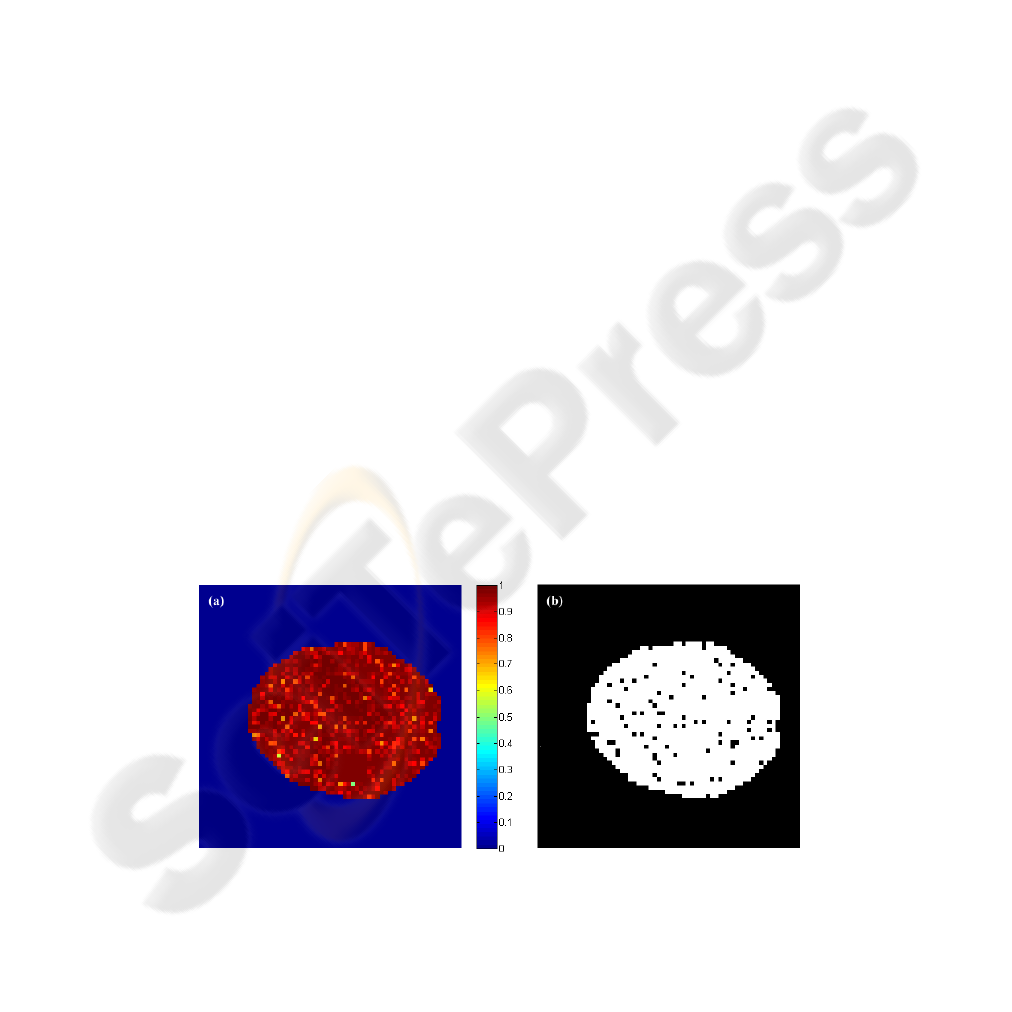
First, we calculate Shannon’s entropy for each voxel of the simulated data. The values
of entropy for the 1398 voxels contained in the interior of the artificial brain had varied
of 0.4949 to 1, where the 49 voxels with activation signal had presented one high value
of entropy (Figure 2a). After that, about 6% of 1398 voxels were eliminated from the
input data of SOM, these voxels had presented a value of entropy H < 0.85 (Figure
2b).
Fig.2. (a) Entropic map of the artificial data; (b) Entropic analysis of synthetic data. The dark
dots in the image were eliminated, the equivalent of 6% of the input data.

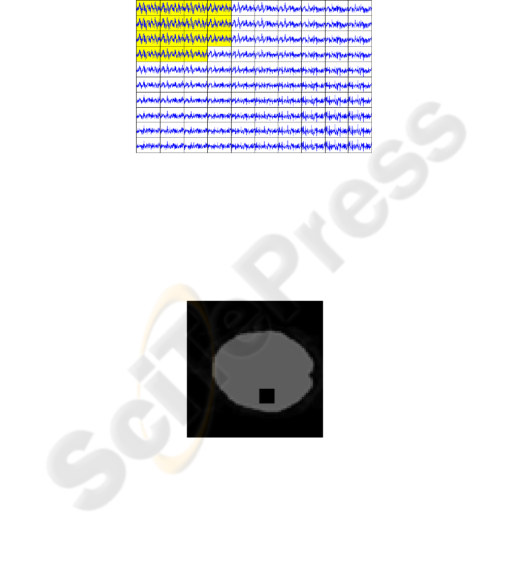
From the final conformation of the neuronal grid achieved after 100 algorithm itera-
tions (Figure 3), we can observe that voxels with similar temporal patterns are clustered
together in the SOM.
Fig.3. 10×10 grid of neurons after implementation of the SOM algorithm, the cluster of neurons
in yellow match the patterns of activity.
For better visualization of these clusters, there are several clustering methods that
can be used, such as K-means [23], fuzzy logic [24] and correlation as a measure of
similarity in a hierarchical clustering [16]. We use this last reference utilizing a simple
correlation as a measure of similarity between neurons in the grid.
Figure 4 shows the active regions defined using the average signal from the neurons
demarcated in the Figure 3. A correlation coefficient (CC) was determined between this
average and each voxel in a fMRI dataset, showing only those with CC > 0.7056.
Fig.4. The dark regions in the brain correspond to active regions as defined by the SOM after
100 iterations.

3.2 Real Data
The same analytical procedure used for simulated data was used to deal with real data.
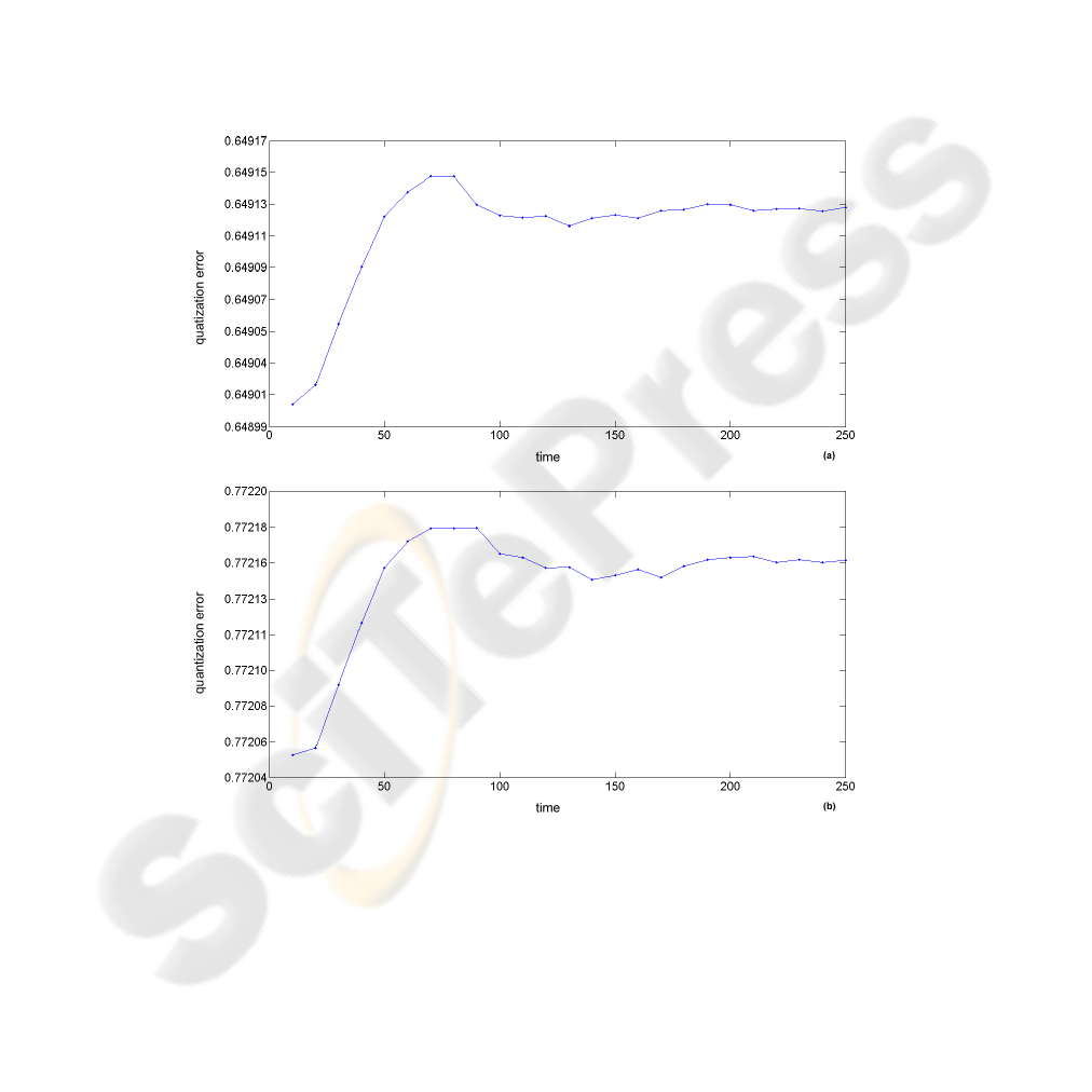
However, we adopted the quantization error (Eq. 8) to estimate the amount of steps of
the algorithm and also act as quality controller of learning. Figure 5 shows the evolution
of error to each 10 iterations, using normalized data. But even if the error has begun to
stabilize at around 100 repetitions, the training is continued until 250 iterations in order
to perform a fine tuning of the map features and thus produce a statistically accurate
quantization of the input space. Analyzing the same figure, it is possible verify that the
magnitude of error for the case where it was applied to analyze the entropic prior to
SOM (Fig. 5a) presents lower, also have begun to stabilize somewhat earlier than the
case where not used the Shannon’s entropy (Fig. 5b).
Fig.5. Graph of the quantization error for a total of 250 iterations. (a) quantization error with the
application of entropy; (b) quantization error without entropy.
Figure 6 reveals the active voxels, according to our method, in the eighth slice of
fMRI data CC > 0.6. In it you can see two main regions as a result of the auditory task
located in the temporal lobe.

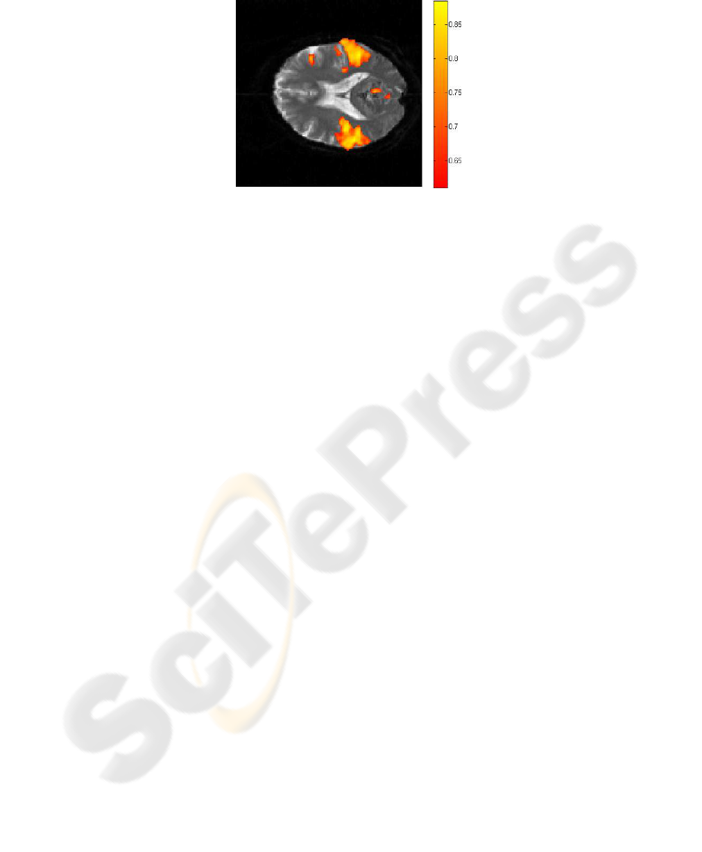
Fig.6. Active regions correlated with the auditory stimulation defined after 250 iterations with
the SOM.
4 Conclusions
The Kohonen’s self-organizing map was applied in data of functional magnetic reso-
nance in synthetic and real models, this last one representing an auditory experiment
with the paradigm in block. With the purpose of increasing the efficiency of the analy-
sis method was proposed to Shannon’s entropy, which eliminated a range of 5 − 10%
of the set of input data. The configuration of the data after the entropy analysis allowed
more likely to find groups of neurons active in the SOM grid with a smaller number of
iterations. Moreover, in the temporal evolution of the quantization error of the SOM, it
can be verified that entropy analysis decreased the amplitude of this error and admitted
his slightly faster stabilization. The results of SOM, both for simulated data, as for real
data, reaffirmed that it can be used as a tool for interpretation of fMRI data. And it has
the advantage that the shaped of the hemodynamic response is not considered, that is, a
HRF modeled mathematically is not used.
References
1. Fontoura, D. R., Ans, M., Costa, J. C., Portuguez, M. W.: Identifying language cerebral func-
tions: a study of functional magnetic resonance imaging in patients with refractory temporal
lobe epilepsy. Journal of Epilepsy and Clinical Neurophysiology, 14(1) (2008) 7-10.
2. Ogawa, S., Lee, T. M., Kay, A. R., and Tank, D. W.: Brain magnetic resonance imaging with
contrast dependent on blood oxygenation. Proceedings of the National Academy of Sciences
of USA, 87 (1990) 9868-9872.
3. Thulborn, K, R., Waterton, J. C., Matthews, P. M., and Radda, G. K.: Oxygenation depen-
dence of the tranverse relaxation time of water protons in whole blood at high field. Biochim-
ica et Biophysica Acta, 714 (1982) 265-270.
4. Pauling, L. and Coryell, C.: The magnetic properties and structure of hemoglobin, oxyhe-
moglobin, and carbon monoxyhemoglobin. Proceedings of the National Academy of Sci-
ences of USA, 22 (1936) 210-216.
5. Huettel S. A., Song A. W., and McCarthy G.: Functional Magnetic Resonance Imaging.
Sinauer Associates, 1st edition (2004).

6. Rabe-Hesketh, S., Bullmore, E., and Brammer, M.: The analysis of functional magnetic res-
onance images. Stat. Methods Med. Res. 6 (1997) 215-237.
7. Friston, K. J., Holmes, A. P., Worsley, K. J., Poline, J. P., Frith, C. D., and Frackowiak, R. S.
J.: Statistical parametric maps in functional imaging: A general linear approach. Hum. Brain
Mapping 2 (1995) 189-210.
8. McKeown, M.J., Makeig, S., Brown, G. G., Jung, T. P., Kindermann, S. S., Bell, A. J., and
Sejnowski, T. J.: Analysis of fMRI data by blind separation into independent spatial compo-
nents. Human Brain Mapping, 6 (1998) 160-168.
9. Biswal, B. B., and Ulmer J. L.: Blind source separation of multiple signal sources of fMRI
data sets using independent component analysis. Journal of Computer Assisted Tomography,
23 (1999) 265-271.k
10. Friston, K. J., Frith, C. D., Liddle, P. F., and Frackowiak, R. S. J.: Functional connectivity:
the principal component analysis of large (PET) datasets. Journal of Cerebral Blood Flow
and Metabolism, 13 (1993) 5-14.
11. Kohonen T.: Self-organized formation of topologically correct feature maps. Biol. Cybernet.
Vol. 43 (1982) 59-69.
12. Friston, K. J., Fletcher, P., Josephs, O. Holmes, A., Rugg, M. D., and Turner, R.: Event-
related fMRI: Characterizing differential responses. NeuroImage, 7 (1998) 30-40.
13. Glover, G. H.: Deconvolution of impulse response in event-related BOLD fMRI. NeuroIm-
age, 9 (1999) 416-429.
14. Chuang K. H., Chiu M. J., Lin C. C., and Chen J. H.: Model-Free functional MRI analysis
using Kohonen clustering neural network and fuzzy C-means. IEEE Transactions on Medical
Imaging, Vol. 18 (1999) 1117-1128.
15. Fischer, H. and Hennig J.: Neural network-nased analysis of MR time series. Magnetic Res-
onance in Medicine, Vol. 41 (1999) 124-131.
16. Liao, W., Chen, H., Yang, Q., Lei, X.: Analysis of fMRI Data Using Improved Self-
Organizing Mapping and Spatio-Temporal Metric Hierarchical Clustering. IEEE Transac-
tions on Medical Imaging, Vol. 27 (2008) 1472-1483.
17. Ngan, S. C. and Hu X.: Analysis of functional magnetic resonance imaging data using self-
organizing mapping with spatial connectivity. Magnetic Resonance in Medicine, vol. 41
(1999) 939-946.
18. Ngan, S. C., Yacoub E. S., Auffernann W. F, and Hu X.: Node merging in Kohonen’s self-
organizing mapping of fMRI data. Artificial Intelligence in Medicine, vol. 25 (2001) 19-33.
19. Peltier, S. J., Polk T. A., Noll D.C.: Detecting low-frequency functional connectivity in fMRI
using a self-organizing map (SOM) algorithm. Hum. Brain Mapp., vol. 20 (2003) 220-226
20. Gibbons, R. D., Lazar, N. A., Bhaumik, D. K., Sclove, S. L., Chen, H. Y., Thulborn, K. R.,
Sweeney, J. A., Hur, K., and Patterson, D.: Estimation and classification of fMRI hemody-
namic response patterns. NeuroImage, 22 (2004) 804-814.
21. de Araujo, D. B., Tedeschi, W., Santos, A. C., Elias, J. Jr., Neves, U. P., Baffa, O.: Shannon
entropy applied to the analysis of event-related fMRI time series. Neuroimage, 20(1) (2003)
311-317.
22. Shannon, C. E.: A mathematical theory of communication. Bell system technical journal 27
(1948) 379-423, 623-656.
23. Goutte, C., Toft, P., Rostrup, E., Nielsen F., A., and Hansen, L. K.: On clustering fMRI time
series. NeuroImage, Vol. 9 (1999) 298-310.
24. Wismuller A., Meyer-Base, A., Lange O., Auer D., Reiser, M. F., and Sumners, DeWitt.:
Model-free functional MRI analysis based on unsupervised clustering. Journal of Biomedical
Informatics 37, (2004) 10-18.