NORMAL FLAT FORMS FOR A CLASS OF 0-FLAT AFFINE

DYNAMICAL SYSTEMS AND ITS APPLICATION TO

NONHOLONOMIC SYSTEMS

S. Bououden, D. Boutat

PRISME - ENSI de Bourges, 10 boulevard Lahitolle, 18020, Bourges cedex, France

F. Abdessemed

Faculty of Engineering, Electronic Departement, Batna University, 05000, Algeria

Keywords:

Flatness, Nonlinear systems, Normal form, Involutivity, Nonholonomic systems.

Abstract:

In this contribution normal ﬂat forms are used to achieve stable tracking control for nonlinear ﬂat systems.

Our approach is based on a nonlinear transformations in order to derive two 0-ﬂat normal forms for a class

of non-linear systems, a dynamical control law is then proposed to achieve stable trajectory tracking. Finally,

This method is generalized to analysis and control a class of a 0-ﬂat afﬁne nonlinear multi-input dynamical

systems for which we can build ﬂat outputs to give structural normal ﬂat forms. The computer simulations are

given in the paper to demonstrate the advantages of the method.

1 INTRODUCTION

The control of nonholonomic dynamic systems has

received considerable attention during the last years

and become a popular subject in the nonlinear con-

trol. One a reasons for this, in real world, the non-

holonomic systems are frequently used to describe

some pratical control systems such as mobile robot,

car-like vehicule, and under-actuated satellites, can

all be modeled as nonholonomic control systems or

nonholonomic maneuvers. Hence, control problems

involve them have attracted attention in the control

community.

Different methods have been applied to solve mo-

tion control problems. (Kanayama et al., 1991) pro-

pose a stable tracking control method for nonholo-

nomic vehicule using a Lyapunov function. (Lee et

al., 1998) solved tracking control using backstepping

and in (Lee and Tai, 2001) with saturation constraints.

Furthermore, most reported designs rely on intelli-

gent control approaches such as Fuzzy Logic Control

(Pawlowski et al., 2001), (Tsai et al., 2004), Neural

Networks (Song and Sheen, 2000), and (Chwa, 2004)

used a sliding mode control to the tracking control

problem. (Fierro and Lewis, 1995) propose a dynam-

ical extention that makes possible the integration of

kinematic and torque controller for a nonholonomic

mobile robot. (Fukao et al., 2000), introduces an

adaptive tracking controller for the dynamic model of

mobile robot with unknown parameters using back-

stepping. However the ﬁeld of control of such sys-

tems is still open to develop other control strategie.

Application of ﬂatness to problems of engineering

interest have grown steadily in recent years. Michel

Fliess et al. (Fliess et al., 1992), (Fliess et al., 1995)

introduced the concept of ﬂat outputs, these outputs

guarantee that the problem will be put in term of con-

trol algorithm for motion planning, trajectory genera-

tion and stabilization. A limitation of ﬂatness is that

there does not exist necessary and sufﬁcient condi-

tions to determine if a general system is differentially

ﬂat and there no algorithm to compute the ﬂat out-

puts. Nevertheless, it is well-known that all control-

lable linear systems can be shown to be ﬂat. Indeed,

any system that can be transformed into a linear sys-

tem by changes of coordinates, static feedback trans-

formations, or dynamic feedback transformations is

also ﬂat (Jakubczyk and Respondek, 1980), (Hunt et

al., 1983).

We present in this paper two normal ﬂat forms, It

deals with sufﬁcient geometrical conditions which en-

able us to conclude if a given nonlinear controllable

dynamical system can be transformed, by means of

change of coordinates, to one of these normal forms.

275

Bououden S., Boutat D. and Abdessemed F. (2010).

NORMAL FLAT FORMS FOR A CLASS OF 0-FLAT AFFINE DYNAMICAL SYSTEMS AND ITS APPLICATION TO NONHOLONOMIC SYSTEMS.

In Proceedings of the 7th International Conference on Informatics in Control, Automation and Robotics, pages 275-280

DOI: 10.5220/0002949002750280

 SciTePress

In the same way it gives an algorithm to compute the

ﬂat outputs. As an illustration to the proposed ap-

proach, a trajectory tracking of a nonholonomic uni-

axial vehicule is simulated. As we will show with this

example, for this particular class, our method presents

a new direction to solve the ﬂatness problem.

The paper is organized as follows. In section 2 we

address notations, deﬁnitions and our problem state-

ment, we describes the classes of 0-ﬂat systems study.

The necessary and sufﬁcient geometrical conditions

for afﬁne dynamical systems are presented in Section

3. In sections 4 provides illustrative examples and

simulations. Some conclusions are presented in sec-

tion 5.

2 DEFINITION AND PROBLEM

STATEMENT

Let us consider the following class of multivariable

nonlinear systems described in state space form by

equations of the following kind In the next section,

we will recall the concept of 0-ﬂat systems

˙x = f (x) +

∑

i=1

(x)u

(1)

where x ∈ χ ⊆ ℜ

, u ∈ U ⊆ ℜ

and f is a smooth

function on χ×U.

Deﬁnition 1. The dynamical system (1) is ﬂat if there

exist m functions y = (y

, ..., y

) called the ﬂat outputs

such that:

1- y = F(x, u, ˙u,..., u

)

) is a function of the state x,

the input u, and its derivatives u

(i)

2- x = ϕ(z, ˙z, ..., z

)

) is a function of the ﬂat outputs

and their derivatives.

3- u = γ(z, ˙z, ..., z

2+1

)

) is a function of the ﬂat out-

puts and their derivatives.

In this paper, we will deal with multi-input afﬁne dy-

namical systems, without loss of generality, we will

assume within this work that:

Assumption 1. The vector ﬁeld G = [g

, ..., g

] is of

rank m.

However, we don’t assume that ∆ = span(G) is invo-

lutive as it is the case in many researches which try to

compute the inverse dynamics. We will characterize a

class of dynamical systems for which the ﬂat outputs

are only functions of states x. This dynamical systems

is called 0-ﬂat: (Pereira, 2000)

= F

(x); where 1 ≤ i ≤ m (2)

2.1 A Class of Structurally 0-Flat

Dynamical System

It is well-known that the codimension one (m = n −

1) controllable dynamical systems are 0-ﬂat (Charlet

and L´evine, 1989). Our result concerns a normal ﬂat

forms of afﬁne dynamical systems with n states and

m = n−2 inputs (codimension 2). Our objective is to

introduce our formulation.

2.2 Main Result

In the sequel we introduce the following notation

= z

j,i

= y

with j = 1 : m relative to the ﬂat out-

put y

, which means i− 1 derivation of the output y

2.2.1 First 0-Flat Normal Form

Let us consider the following proposition written in

terms of the z

, where j = 1 : m state variables. Let

us consider the following proposition

Proposition 1. The following dynamical system is

0-ﬂat

˙z

= z

n−2

∑

i=3

(z)u

˙z

= α

(z) + u

+ β

(z)u

+ ... + β

(z)u

˙z

= z

n−2

∑

i=3

(z)u

(3)

˙z

= α

(z) + β

(z)u

+ u

+ ... + β

(z)u

˙z

= α

+ u

n−2

∑

i=3,i6= j

(z)u

with z

, z

as ﬂat outputs, and m = n− 2.

Proof 1. Now we will show that the equations (3)

represent a locally dynamical 0-ﬂat system. Consider

the following m equations :

= ˙z

1,1

− z

1,2

−

∑

i=3

(z)u

= 0 (4)

= ˙z

2,1

− z

2,2

−

∑

i=3

(z)u

= 0 (5)

= ˙z

j,1

− α

j,1

− u

−

∑

i=3,i6= j

(z)u

= 0 (6)

where 3 ≤ j ≤ m

Let v = (z

1,2

, z

2,2

, u

, ..., u

) be the vector of un-

known system variables and let us compute the fol-

lowing partial derivative

∂(E

, ..., E

)

∂v

= −I

+ O (v) (7)

ICINCO 2010 - 7th International Conference on Informatics in Control, Automation and Robotics

276

Where I

is the identity matrix and O (v) represents

the order one of the v variables. From the equations

(4, 5, 6) and the fact that

∂(E

,...,E

)

∂v

is locally invert-

ible then the implicite function theorem, allows us to

conclude that there exists ϕ

() and γ

() functions such

that

k,2

= ϕ

, ˙y

, j = 1 : m, k = 1 : 2) (8)

= γ

, ˙y

, j = 1 : m, k = 3 : m) (9)

By replacing (8) and (9) in the second and the fourth

dynamic equation of (3) we can get the inputs u

and

as functions of (y

, ˙y

) for j = 1 : m and their sec-

ond derivatives y

(2)

, y

(2)

. In the next subsection we

will give a slightly different 0-ﬂat normal form which

is related to more drastic conditions.

2.2.2 Second 0-Flat Normal Form

The second canonical system gives the missing vari-

ables from the successive derivation of the same ﬂat

output written in terms of the variables z

= y

, 1 ≤

j ≤ (n− 2) :

Proposition 2. The following dynamical system is

0-ﬂat

˙z

= z

n−2

∑

i=2

(z)u

˙z

= z

n−2

∑

i=2

(z)u

(10)

˙z

= α

(z) + u

n−2

∑

i=2

(z)u

˙z

= α

j1(z)

+ u

n−2

∑

i=2

(z)u

Where 2 ≤ j ≤ m, and m = n − 2.

Proof 2. The main difference from (3) concerns the

fact that we assume the variable z

not present in the

dynamics ˙z

, for 1 ≤ j ≤ (n − 2). Then we can con-

clude that

Condition 1. z

must not be present in β

(z) for

j = 1 : m, and i = 2 : m

Condition 2. z

must not be present in α

for

j = 2 : m.

Under these conditions we can use the same proce-

dure as the canonical form (3) to solve the dynamical

system (10). So let us consider the m equations:

= ˙z

− z

−

n−2

∑

i=2

(z)u

= 0 (11)

= ˙z

− α

j1(z)

− u

−

n−2

∑

i=2

(z)u

= 0 (12)

We can put v = (z

, u

, ..., u

) the vector of un-

known system variables. Let us compute the follow-

ing partial derivative

∂(E

, E

..., E

)

∂v

= −I

+ O

(v) (13)

Where I

is the identity matrix and O

(v) represents

the order one of the v variables. From the equations

(11, 12) and the fact that

∂(E

,...,E

)

∂v

is locally in-

versible then the implicite function theorem, allows

us to conclude that there exists ϕ

() and γ

() func-

tions such that

1,2

= ϕ

, ˙y

, j = 1 : m) (14)

= γ

, ˙y

, j = 1 : m, k = 2 : m) (15)

By replacing (14) and (15) in the second and the

third dynamic equation of (10) we can get the variable

as a function of ˙y

, y

(2)

and y

for i = 1 : m. Also

we get the input variable u

as a function of ˙y

, y

(2)

(3)

and y

for i = 1 : m.

3 TRANSFORMATIONS

Now, we give some conditions for a class of nonlinear

systems, for which we can transform a nonlinear dy-

namical system (1) in a new 0-ﬂat normal forms. So

we distinguished two cases:

Case 1. The controllability distribution has the

following vector ﬁeld:

∆

= span{g

, g

, ..., g

n−2

, ad

}, with

dim(∆

) = n.

Case 2. The controllability distribution has the

following:

∆

= span{g

, g

, ..., g

n−2

, ad

}, with

dim(∆

) = n.

3.1 Case 1

Proposition 1. If the distribution ∆

span{g

, g

} ⊆ ∆

is involutive, then the dynamical

system (1) is 0-ﬂat.

Proof 1. As dim(∆

) = n and ∆

is a 2-dimensional

involutive distribution, there exist n− 2 = m indepen-

dent functions of states x, (y

= z

i,1

), 1 ≤ i ≤ m such

that:

• ∆

i=1

kerdy

where kerdy

means the kernel

of the differential of the function y

NORMAL FLAT FORMS FOR A CLASS OF 0-FLAT AFFINE DYNAMICAL SYSTEMS AND ITS APPLICATION TO

NONHOLONOMIC SYSTEMS

277

• L

, f]

k,1

= 1 for k = 1 : 2

• L

k,1

= 1 for 3 ≤ k ≤ m

Now let us consider for k = 1 : 2 the following new

variables: z

k,2

= L

k,1

where L

is the Lie derivative

in the direction of f. Therefore the set of the n vari-

ables: (z

i,1

), 1 ≤ i ≤ m, z

1,2

and z

2,2

form a new co-

ordinate system. For this the derivative of these vari-

ables give structural 0-ﬂat normal form (3).

3.2 Case 2

Now let us describe the above conditions (1), (2) in

(Proof 2) geometrically. For this one remarks that in

(10) we have g

∂

∂z

1,3

. Therefore the independence

of the others input directions (g

)

2≤i≤m

from the vari-

ables z

1,3

can be described by the fact that:

, g

, ] ∈ span{g

, ad

Indeed ad

∂

∂z

1,3

+ h(z)

∂

∂z

1,2

. For second condi-

tion, α

j,1

= L

j,1

for all j ≥ 2. Then, if we want

this function independent of the variable z

1,3

, then we

must have L

j,1

= 0. As u

is not present in the

last equations of (10) then L

j,1

= 0. Therefore,

j,1

= 0 is equivalent to L

j,1

= 0. Thus we

can conclude that the distribution ∆

= {g

, ad

} is

involutive.

Proposition 3. If the distribution ∆

= {g

, ad

} ⊆

∆

is involutiveand [g

, g

] ∈ span{g

} then the

dynamical system (1) is 0-ﬂat.

4 ILLUSTRATIVE EXAMPLE

In order to verify the performance of proposed

methodology, as an illustration, we used a nonholo-

nomic system. A nonlinear transformation is made in

order to derive a 0-ﬂat normal forms, the results ob-

tained with our proposed control based on 0-ﬂat nor-

mal forms of codimension 2 are used to control the

nonlinear system in the aim to show its usefulness.

4.1 Application to a Nonholonomic

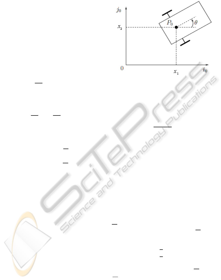
Uniaxal Vehicule

The example we study is the kinematic model of

a mobile car (see Figure 1), this system can be

represented by the following set of equations:







˙x

= vcosθ

˙x

= vcosθ

θ = ω

(16)

Figure 1: Coordinates system of car.

where

, x

) represents the cartesian position of the centre

of mass of the car,

θ its inclination with respect to the horizontal axis,

(v, ω) its forward and angular velocities respectively.

the model (16) is not static feedback linearizable.

However, the problem can be solved by introducing

the new state x

˙x

+ ˙x

Resulting in the extended static feedback linearizable

system described by:











˙x

= x

cos(x

)

˙x

= x

sin(x

)

˙x

= u

˙x

= u

(17)

The outputs are the states variables: x

, x

), the above equations can be written in

the following form:

˙x = f (x) + g

(x)u

+ g

(x)u

; (18)

where f(x), g

(x), g

(x) are the smooth vector ﬁelds.

We will transform the nonlinear dynamical system

(17) in a structural 0-ﬂat normal form, the distribu-

tion

∆

= {g

, g

} has dimension 2.

The bracket [g

, g

] = 0 which means that ∆

is invo-

lutive. Then there exists two functions y

(x) and y

(x)

such that:

(x).∆

= 0 (19)

(x).∆

= 0 (20)

From (19) and (20) we can conclude that

∂y

∂x

= 0 and

∂y

∂x

= 0 ∀x

, x

. Then it is enough to set y

(x) a func-

tion of x

and y

(x) any function in terms of x

. Let

us consider y

= x

and y

= x

Now let us consider for k = 1 : 2 the following vari-

ables: z

k,1

= y

and the new coordinate variables:

1,2

= L

1,1

and z

2,2

= L

2,1

ICINCO 2010 - 7th International Conference on Informatics in Control, Automation and Robotics

278

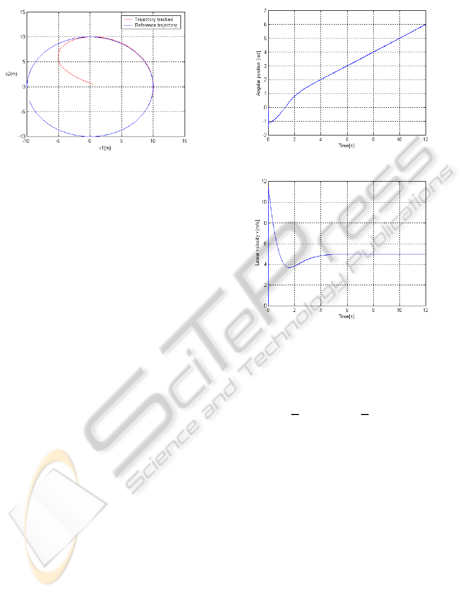
Figure 2: Trajectory tracked by uniaxal vehicule.

For this the derivativeof these variablesgive struc-

tural 0-ﬂat normal form (3).

˙z

= z

n−2

∑

i=3

(z)u

˙z

= α

(z) + u

+ β

(z)u

+ ... + β

(z)u

˙z

= z

n−2

∑

i=3

(z)u

(21)

˙z

= α

(z) + β

(z)u

+ u

+ ... + β

(z)u

The system is codimension 2, the canonical form can

be expressed as follows:











˙z

= z

˙z

= α

(z) + β

(z)u

+ β

(z)u

˙z

= z

˙z

= α

(z) + β

(z)u

+ β

(z)u

(22)

where

= 0, α

= 0

(z) = x

sin(x

);β

(z) = x

cos(x

)

(z) = cos(x

);β

(z) = sin(x

)

The main objective of the ﬂatness based controller

is to obtain the asymptotic tracking of a desired tra-

jectory, let the system output be y

= z

, y

= z

from (22) we can obtain the expressions of u

, u

terms of (y

, ˙y

, y

, ˙y

), and the second derivatives of

two ﬁrst variables ¨y

, ¨y

. Let ¨y

= v

, ¨y

= v

two

new inputs control such that:







¨y

+ k

( ˙y

− ˙y

) + k

− y

)

¨y

+ k

( ˙y

− ˙y

) + k

− y

)



where k

, k

> 0 are control gains chose care-

fully to ensure exponential stability, and ¨y

, ˙y

, y

are

prescribed reference trajectories.

The control law:







(z) β

(z)

(z) β

(z)



−1



− α

(z)

− α

(z)



The controller gains are chosen to be:

Figure 3: Unicycle orientation x

Figure 4: Linear velocity of unicycle vehicule.

= diag[1000, 1000], k

= diag[1000, 1000].

We consider the following continuously derivable

desired trajectories:

= rsin

t, y

= −rcos

t is assigned, which

described a circular movement with radius r = 10 at

the constant speed v

= 5.

The closed loop system was simulated using the

initial conditions x

(0) = (0.5;0.5;0;0.1) for system

(17).

The trajectory tracked (see Fig. 2) is very close

to the desired one, achieving by thus the control ob-

jective. Finally, angular position and linear velocity

are depicted in the Fig. 3 and Fig. 4. It can be seen

that our control scheme achieves satisfactory perfor-

mances.

5 CONCLUSIONS

We described the development of a tracking controller

based on normal ﬂat forms. This method is general-

ized to analysis and control a class of a 0-ﬂat afﬁne

nonlinear multi-input dynamical systems for which

NORMAL FLAT FORMS FOR A CLASS OF 0-FLAT AFFINE DYNAMICAL SYSTEMS AND ITS APPLICATION TO

NONHOLONOMIC SYSTEMS

279

we can build ﬂat outputs to give structural normal ﬂat

forms. Simulation results show an acceptable perfor-

mance under the studied cases.

REFERENCES

Fliess, M., L´evine, J., Martin, P. and Rouchon, P., 1992. Sur

les systmes non linaires diffrentiellement plats. C. R.

Acad. Sci. Paris Sr. I Math., 315: pp 619-624.

Fliess, M., L´evine, J., Martin, P. and Rouchon, P., 1995.

Flatness defect of non-linear systems introductory the-

ory and examples. Internat. J. Control, 61: pp 1327-

1361.

Chwa, D., 2004. Sliding- Mode Tracking Control of non-

holonomic Wheeled Mobile robotin polar coordinates,

IEEE Trans. On Control Syst. Tech. Vol. 12, No. 4,pp

633-644.

Fierro, R., Lewis, F. L., 1995. Control of Nonholonomic

Mobile Robot: Backstepping Kinematics into Dynam-

ics, Proc. 34th Conf. On Decision & Control, New

Orleans, LA.

Fukao, T., Nakagawa, N. Adachi, 2000. Adaptive Track-

ing Control of a Nonholonomic Mobile Robot. IEEE

Trans, On Robotics and Automation, Vol. 16, No. 5,

pp609-615.

Kanayama, Y., Kimura, Y., Miyazaki, F., Noguchi, T.

1991. A stable Tracking control method for a

Non-Holonomic Mobile Robot. Proc. IEEE/RSJ Int.

Workshop on Intelligent Robots and Systems, Osaka,

Japan, pp 1236-1241.

Lee, T-C., Lee, C.H., Teng, C-C. 1998. Tracking Control

of Mobile Robots Using the Backsteeping Technique,

Proc. 5th. Int. Conf. Contr., Automat Robot. Vision,

Singapore, pp 1715-1719.

Lee, T-C., Tai, K., 2001. Tracking Control of Unicycle

Modeled Mobile robots using a saturation feedback

controller, IEEE Trans. On Control Systems Technol-

ogy, Vol. 9, No. 2, pp 305-318.

Pawlowski, S., Dutkiewicz, K. Kozlowski, Wroblewski, W.,

2001. Fuzzy logic implementation in Mobile robot

Control, 2th Workshop On Robot Motion and Control,

pp 65-70.

Tsai, C-C., Lin, H-H, Lin, C-C., 2004. Trajectory Track-

ing control of a Laser-Guided wheeled mobile robot,

Proc. IEEE Int. Conf. On Control Application, Taipei,

Taiwan, pp 1055-1059.

Song, K. T., Sheen, L. H., 2000. Heuristic fuzzy-neural

Network and its application to reactive navigation of

a mobile robot, Proc. IEEE Int. Conf. On Control Ap-

plication, Taipei, Taiwan, pp 1055-1059.

Pereira da Silva., 2000. Flatness of nonlinear control sys-

tems a Cartan-K¨ahler approach, In Proc. Mathemat-

ical Theory of Networks et Systems MTNS’2000,

pages 1 10, Perpignan, Jun. 19-23.

Jakubczyk, B., Respondek, W., 1980. On linearization of

control systems, Bull. Acad. Pol. Sc., Ser. Sci. Math.,

28: pp 517-522.

Hunt, L. R., Su, R. and Meyer, G., 1983. Global transfor-

mations of nonlinear systems, IEEE Trans. Automat.

Control, 28:24-31.

Charlet, B., L´evine. J., On dynamic feedback linearization,

Systems Control Lett., 13: pp 143-151.

ICINCO 2010 - 7th International Conference on Informatics in Control, Automation and Robotics

280