A NEW PREDICTOR/CORRECTOR PAIR TO ESTIMATE THE
VISUAL FEATURES DEPTH DURING A VISION-BASED
NAVIGATION TASK IN AN UNKNOWN ENVIRONMENT
A Solution for Improving the Visual Features Reconstruction During an Occlusion
A. Durand Petiteville, M. Courdesses and V. Cadenat
CNRS, LAAS, 7 avenue du colonel Roche, F-31077 Toulouse, France
Universit
´
e de Toulouse, UPS, INSA, INP, ISAE, LAAS, F-31077 Toulouse, France
Keywords:
Visual servoing, Visual data estimation, Predictor/estimator pair.
Abstract:
This papers deals with the problem of estimating the visual features during a vision-based navigation task
when a temporary total occlusion occurs. The proposed approach relies on an existent specific algorithm.
However, to be efficient, this algorithm requires highly precise initial values for both the image features and
their depth. Thus, our objective is to design a predictor/estimator pair able to provide an accurate estimation of
the depth value, even when the visual data are noisy. The obtained results show the efficiency and the interest
of our technique.
1 INTRODUCTION
In the past decades, many works have addressed
the problem of using information provided by a vi-
sion system to control a robot. Such techniques are
commonly known as Visual Servoing (Corke, 1996),
(Chaumette and Hutchinson, 2006). Visual servoing
is roughly classified into two main categories: Im-
age based visual servoing (IBVS) and Position based
visual servoing (PBVS) (Chaumette and Hutchinson,
2006). In the first approach, the goal to be reached
is expressed only in the image space, whereas in the
second one, it is given in terms of a desired camera
pose (Corke, 1996). A complete survey can be found
in (Chaumette and Hutchinson, 2006).
We focus in the sequel on the first kind of con-
trol. In this case, the control law depends only on the
visual features. Therefore, if they are lost because
of an occlusion or any other unexpected event, the
desired task cannot be realized anymore. Here, we
are working in a mobile robotics context. In this con-
text, the realization of a vision-based navigation task
in a given environment requires to preserve not only
the image data visibility, but also the robot safety.
In that case, techniques allowing to avoid simultane-
ously collisions and visual data losses appear to be
limited, because they are restricted to missions where
an avoidance motion exists without leading to local
minima (Folio and Cadenat, 2008). As many robotic
tasks cannot be performed if the visual data loss is not
tolerated, it is necessary to provide methods which
accept that occlusions may effectively occur without
leading to a task failure.
Folio has proposed such an approach (Folio and
Cadenat, 2008). The idea is to reconstruct the vi-
sual features whenever necessary. The developed al-
gorithm is based upon the vision/motion link which
relates the variation of the visual features in the im-
age to the camera motion. However, this method
needs accurate initial values for the visual features
and the depth. If the first ones can be obtained from
the last image available before the occlusion occurs,
determining a precise initial value for the depth suf-
ficiently rapidly to correctly handle the occlusion re-
mains a challenging problem. Different approaches
are proposed in the literature. See for instance the
works by Matthies who derived and compared several
algorithms based on a Kalman filter (Matthies et al.,
1989). However, a correct depth value can be ob-
tained only if the camera motion respects some very
particular constraints. These solutions are not suit-
able for our particular case. It would be also possible
to use the epipolar geometry (Ma et al., 2003), stere-
ovision (Cervera et al., 2002), or even structure from
motion techniques (Jerian and Jain, 1991). However,
this kind of approaches are time-consuming and can-
268
Durand Petiteville A., Courdesses M. and Cadenat V. (2010).
A NEW PREDICTOR/CORRECTOR PAIR TO ESTIMATE THE VISUAL FEATURES DEPTH DURING A VISION-BASED NAVIGATION TASK IN AN
UNKNOWN ENVIRONMENT - A Solution for Improving the Visual Features Reconstruction During an Occlusion.
In Proceedings of the 7th International Conference on Informatics in Control, Automation and Robotics, pages 268-274
DOI: 10.5220/0002948902680274
Copyright
c
 SciTePress

not be used for our purpose. Finally, (De Luca et al.,
2008) have proposed to estimate the depth using a non
linear observer. But, unfortunately, the convergence
time seems to be too large to be useful in our specific
context.
In this paper, we have developed a non recursive
algorithm based on a predictor/corrector pair allowing
to provide an accurate value of the depth using visual
data. This value will then be used to feed D. Folio’s
algorithm in order to improve its efficiency.
The paper is organized as follows. Section II is
dedicated to some preliminaries regarding the system
modelling, the visual servoing control law design and
the description of D. Folio’s algorithm. Section III de-
tails and analyzes the predictor/estimator pair which
has been developed. Finally, simulation results vali-
dating our approach are shown in section IV.
2 PRELIMINARIES
2.1 System Modelling
We consider the system presented in figure 1(a),
which consists of a robot equipped with a cam-
era mounted on a pan-platform. We describe
the successive frames : F
O
(O,~x
O
,~y
O
,~z
O
) attached
to the world, F
M
(M,~x
M
,~y
M
,~z
M
) linked to the
robot, F
P
(P,~x
P
,~y
P
,~z
P
) attached to the platform, and
F
C
(C,~x
C
,~y
C
,~z
C
) linked to the camera. Let θ be the
direction of the robot wrt. ~x
O
, ϑ the direction of the
pan-platform wrt. ~x
M
, P the pan-platform centre of
rotation and D
x
the distance between the robot refer-
ence point M and P. Defining vector q = (l,θ,ϑ)
T
where l is the robot curvilinear abscissa, the control
input is given by ˙q = (υ,ω,ϖ)
T
, where υ and ω are
the cart linear and angular velocities, and ϖ is the pan-
platform angular velocity wrt. F
M
. For such a robot,
the kinematic model is classically given by the fol-
lowing relations:









˙
M
x
(t) = υ(t) cos(θ(t))
˙
M
y
(t) = υ(t) sin(θ(t))
˙
θ(t) = ω(t)
˙
ϑ(t) = ϖ(t)
(1)
where
˙
M
x
(t) is the speed of M wrt. ~x
O
and
˙
M
y
(t) wrt.
~y
O
.
The camera motion can be described by the kine-
matic screw T
C/F
O
:
T
C/F
O
=

(V
C/F
O
)
T
(Ω
F
C
/F
O
)
T
)

T
(2)
where V
C/F
O
and Ω
F
C
/F
O
are the camera translation
and rotation speeds wrt. the frame F
O
. For this spe-
(a) The robotic system. (b) The camera pinhole model.
Figure 1: System modeling.
cific mechanical system, T
C/F
O
is related to the con-
trol input by the robot jacobian J : T
C/F
O
= J ˙q. As
the camera is constrained to move horizontally, it
is sufficient to consider a reduced kinematic screw
T
r
= (V
~y
C
,V
~z
C
,Ω
~x
C
)
T
, and a reduced jacobian matrix
J
r
as follows:
T
r
= J
r
˙q (3)
Defining C
x
and C
y
as the coordinates of C along axes
~x
P
and ~y
P
(see figure 1(a)), J
r
is given by:
J
r
=



−sin(ϑ(t)) D
x
cos(ϑ(t)) +C
x
C
x
cos(ϑ(t)) D
x
sin(ϑ(t)) −C
y
−C
y
0 −1 −1



(4)
It should be noted that J
r
can be inverted (det(J
r
) =
D
x
).
2.2 The Vision-based Navigation Task
The vision-based navigation task consists in position-
ing the camera with respect to a given static landmark.
We assume that this landmark can be characterized
by n interest points which are extracted by our image
processing. Therefore, the visual data are represented
by a 2n-dimensional vector s made of the coordinates
(X
i
,Y
i
) of each point P
i
, in the image plane as shown
on figure 1(b). For a fixed landmark, the variation of
the visual signal ˙s is related to the reduced camera
kinematic screw T
r
thanks to the interaction matrix
L
(s,z)
as shown below (Espiau et al., 1992):
˙s = L
(s,z)
T
r
= L
(s,z)
J
r
˙q (5)
In the case of n points, L
(s,z)
= [L
T
(P
1
)
,...,L
T
(P
n
)
]
T
where L
(P
i
)
is classically given by (Espiau et al.,
1992):
L
(P
i
)
=

L
x
(s
i
,z
i
)
L
y
(s
i
,z
i
)

=
0
X
i
z
i
X
i
Y
i
f
−
f
z
i
Y
i
z
i
f +
Y
2
i
f
!
(6)
where z
i
represents the depth of the projected point
p
i
, and f is the camera focal (see figure 1(b)). At the
A NEW PREDICTOR/CORRECTOR PAIR TO ESTIMATE THE VISUAL FEATURES DEPTH DURING A
VISION-BASED NAVIGATION TASK IN AN UNKNOWN ENVIRONMENT - A Solution for Improving the Visual
Features Reconstruction During an Occlusion
269

beginning of the visual servoing, z
i
is not available
yet. Thus, only an approximation of the interaction
matrix noted
ˆ
L
(s
∗
,z
∗
)
computed at the desired position
will be used to build the control law as in (Chaumette
and Hutchinson, 2006).
To perform the desired vision-based task, we ap-
ply the visual servoing technique given in (Espiau
et al., 1992) to mobile robots as in (Pissard-Gibollet
and Rives, 1995). The proposed approach relies on
the task function formalism (Samson et al., 1991) and
consists in expressing the visual servoing task by the
following task function to be regulated to zero:
e = C(s − s
∗
) (7)
where s
∗
represents the desired value of the im-
age data. Matrix C, called combination matrix, al-
lows to take into account more visual features than
available degrees of freedom. Several choices are
possible: see for example (Comport et al., 2004).
A classical idea consists in defining C =
ˆ
L
+
(s
∗
,z
∗
)
=
(
ˆ
L
T
(s
∗
,z
∗
)
ˆ
L
(s
∗
,z
∗
)
)
−1
ˆ
L
T
(s
∗
,z
∗
)
because the expression of
the control law is simplified (see (8) hereafter). Now,
it remains to determine a controller allowing to make
e vanish. Such a controller is classically designed by
imposing an exponential decrease, that is ˙e = −λe,
where λ is a positive scalar or a positive definite ma-
trix. Then, the visual servoing controller can be writ-
ten as follows:
˙q
(s)
= −(C
ˆ
L
(s
∗
,z
∗
)
J
r
)
−1
λC(s − s
∗
) = J
−1
r
λC(s − s
∗
)
(8)
2.3 Visual Data Estimation
However, the above controller can only be used if the
visual data are available. If they are not because of a
landmark occlusion or a camera failure for example,
the task cannot be realized anymore. To remedy this
critical situation, (Folio and Cadenat, 2008) has re-
cently proposed to solve the dynamic system (5) to
obtain the expression of the visual data. However,
the latter depends not only on s but also on depth z
which must then be determined. As our robot is not
equipped with any sensor able to measure this data,
we have to reconstruct it. After some computations
(see (Folio and Cadenat, 2008) for a detailed proof),
it can be shown that, for any t ∈ [t
k−1
,t
k
], X
i
, Y
i
and z
i
express as:



























X
i
(t) =
z
i
(k−1)X
i
(k−1)
z
i
(t)
Y
i
(t) =
f
z
i
(t)
n
D
x
sin(ϑ(t)) +
υ(k−1)
ω(k−1)
cos(ϑ(t)) −C
y
+c
1
cos(A( ˙q(k − 1))(t − t
k−1
))
−c
2
sin(A( ˙q(k − 1))(t − t
k−1
)
}
z
i
(t) = −D
x
cos(ϑ(t)) +
υ(k−1)
ω(k−1)
sin(ϑ(t)) −C
x
+c
1
sin(A( ˙q(k − 1))(t − t
k−1
))
+c
2
cos(A( ˙q(k − 1))(t − t
k−1
))
(9)
where:

















A( ˙q(k − 1)) = ω(k − 1) + ϖ(k − 1)
c
1
=
Y
i
(k−1)z
i
(k−1)
f
− D
x
sin(ϑ(k − 1))
−
υ(k−1)
ω(k−1)
cos(ϑ(k − 1)) +C
y
c
2
= z
i
(k − 1) + D
x
cos(ϑ(k − 1))
−
υ(k−1)
ω(k−1)
sin(ϑ(k − 1)) +C
x
Thanks to (9), Folio has developped a recursive algo-
rithm able to estimate X
i
,Y
i
and z
i
provided that ϑ(t)
has been previously determined
1
. However, it should
be noted that initial conditions, namely X
i
(k − 1),
Y
i
(k − 1) and z
i
(k − 1), are required to determine
X
i
(k), Y
i
(k) and z
i
(k). So, this algorithm cannot be
used to properly estimate z
i
(k) without a precise ini-
tial value of z
i
(k − 1).
3 METHODOLOGY
In this paper, we propose to estimate the depth by
building a predictor/estimator pair using data from m
images, with m ∈ N
∗
to repair a too small signal/noise
ratio (Durand Petiteville et al., 2009). Our first objec-
tive is to express a predictor
ˆ
X
i
(k|k − j),
ˆ
Y
i
(k|k − j) of
one point P
i
at instant k using the image at k − j, with
j ∈ [1,...,m]. To this aim, we rewrite equation (9) to
relate z
i
(k − 1|k − 1) and z
i
(k|k − 1). We obtain:
ˆz
i
(k − 1|k − 1) =
ˆz
i
(k|k − 1) − β
α
i
(10)
where α
i
and β are given in the appendix. Denoting
by
˜
X
i
(k − 1) and
˜
Y
i
(k − 1) the visual data measured at
instant k −1, we use (10) in (9) to obtain the following
predictor for the visual features:
1
As one can see, solution (9) requires the determination
of ϑ(t). This angle can be simply computed by integrating
˙
ϑ = ϖ between t
k−1
and t. A straightforward calculus leads
to ϑ(t) = ϖ(k − 1)(t − t
k−1
) + ϑ(k − 1), where ϑ(k − 1) is
the pan-platform angular value at t
k−1
, which is usually pro-
vided by the embedded encoder.
ICINCO 2010 - 7th International Conference on Informatics in Control, Automation and Robotics
270














ˆ
X
i
(k|k − 1) =
ˆz
i
(k|k−1)
˜
X
i
(k−1)−β
˜
X
i
(k−1)
ˆz
i
(k|k−1)α
i
ˆ
Y
i
(k|k − 1) =
f
ˆz
i
(k|k−1)
(
˜
Y
i
(k−1)ˆz
i
(k|k−1)
f α
i
cos(A( ˙q(k − 1))T )
−
ˆz
i
(k|k−1)
α
i
sin(A( ˙q(k − 1))T ) + κ
i
)
(11)
where κ
i
is given in the appendix T = t
k
− t
k−1
.
As shown by (11), the obtained predictor depends
only on the last image. To use more than one im-
age and improve the accuracy, a first natural solution
is to recursively use equations (10) and (11). How-
ever, this would lead to highly complex relations.
This is the reason why we propose to find how im-
age k − j can be transformed into image k. Defin-
ing X (k) = [M
x
(k), M
y
(k), θ(k),ϑ(k)]
T
as the system
state at k, we propose to compute the smallest se-
quence of control inputs allowing to reach state at
k starting from state at k − j. To this aim, we first
need to verify the controllability of the corresponding
nonlinear discrete system X (k + 1) = g(X (k), ˙q(k))
where g(X (k), ˙q(k)) is obtained by analytically solv-
ing equation (1). Its expression is given by:
g :















M
x
(k) = M
x
(k − 1)
+
υ(k−1)
ω(k−1)
(sin(θ(k − 1) + ω(k − 1) ∗ T )
−sin(θ(k − 1)))
M
y
(k) = M
y
(k − 1)
−
υ(k−1)
ω(k−1)
(cos(θ(k − 1) + ω(k − 1) ∗ T )
−cos(θ(k − 1)))
θ(k) = θ(k − 1) + ω(k − 1) ∗ T
ϑ(k) = ϑ(k − 1) + ϖ(k − 1) ∗ T















(12)
when ω 6= 0 (the problem is straightforward if ω = 0).
Such a system is controllable in p steps if the follow-
ing matrix P is full rank (Djeridane, 2004).
P =












∂g(X (p−1), ˙q(p−1))
∂ ˙q(p−1)
∂g(X (p−1), ˙q(p−1))
∂X (p−1)
∂g(X (p−2), ˙q(p−2))
∂ ˙q(p−2)
...
∂g(X (p−1), ˙q(p−1))
∂X (p−1)
...
∂g(X (1), ˙q(1))
∂X (1)
∂g(X (0), ˙q(0))
∂ ˙q(0)












T
(13)
It can be shown that P is not full rank for p = 1.
For p = 2, this property is fulfilled if ω 6= 2ηπ for
η ∈ N. Now, thanks to (12), we can compute the two
control inputs allowing to reach the system state at k
from the one at k − j. The first one aims at position-
ning the robot at [M
x
(k), M
y
(k)].
The second one orientates the robot and the plat-
form towards [θ(k),ϑ(k)]. We obtain the following
equations:





υ
e1
=
ω
e1
2sin(
ω
e1
∗T
2
)
∗ R
ω
e1
=
−2θ(k− j)
T
+ 2 arctan

(M
y
(k)−M
y
(k− j))
(M
x
(k)−M
x
(k− j))

ϖ
e1
= 0





υ
e2
= 0
ω
e2
=
θ(k)−(θ(k− j)+ω
e1
T )
T
ϖ
e2
=
ϑ(k)−ϑ(k− j)
T
(14)
where:
R =
q
(M
x
(k) − M
x
(k − j))
2
+ (M
y
(k) − M
y
(k − j))
2
.
Now, thanks to the two control inputs ˙q
e1
=
(υ
e1
,ω
e1
,ϖ
e1
)
T
and ˙q
e2
= (υ
e2
,ω
e2
,ϖ
e2
)
T
given by
(14), we are able to reach the image at instant k from
any image at k − j. It should be noted that the robot
trajectory in the world frame computed with [ ˙q
e1
, ˙q
e2
]
is not the same as the one calculated with the sequence
[ ˙q(k − j),..., ˙q(k − 1)]. Therefore we have to intro-
duce an intermediate state X ( j
0
) to compute our pre-
dictor. It corresponds to the system state which has
been reached at the virtual instant j
0
by applying ˙q
e1
.
Using (10) recursively, we obtain the following re-
sults:
ˆz
i
(k − j
0
|k − j) = ˆz
i
(k − j|k − j)φ
i
+ ϕ
i
ˆz
i
(k|k − j
0
) = ˆz
i
(k − j
0
|k − j)φ
0
i
+ ϕ
0
i
ˆz
i
(k|k − j) = ˆz
i
(k − j|k − j)µ
i
+ ν
i
(15)
The different parameters φ
i
,ϕ
i
,φ
0
i
,ϕ
0
i
,µ
i
,ν
i
and κ
i
in-
volved in these equations are given in the appendix.
Now, using (15) and (11), we express a predictor us-
ing image at k − j as follows:













ˆ
X
i
(k|k − j) =
˜
X
i
(k− j)ˆz
i
(k|k− j)−ν
i
ˆz
i
(k|k− j)µ
i
ˆ
Y
i
(k|k − j) = f
n
˜
Y
i
(k− j)cos(A( ˙q
e1
)T )cos(A( ˙q
e2
)T )
f µ
i
−
sin(A( ˙q
e1
)T )cos(A( ˙q
e2
)T )
µ
i
−
sin(A( ˙q
e2
)T )
φ
0
i
+
γ
i
ˆz
i
(k|k− j)
)
o
(16)
Once the predictors have been obtained, in a second
step, we address the estimators determination prob-
lem. To this aim, we propose to minimize the follow-
ing criterion which represents the error (for one point
P
i
) between the above predictors and the correspond-
ing measures at instant t
k
. We get:
C
∗
=
m
∑
j=1
(
ˆ
X
i
(k|k − j)−
˜
X
i
(k))
2
+(
ˆ
Y
i
(k|k − j)−
˜
Y
i
(k))
2
(17)
Derivating this cost function with respect to the depth
A NEW PREDICTOR/CORRECTOR PAIR TO ESTIMATE THE VISUAL FEATURES DEPTH DURING A
VISION-BASED NAVIGATION TASK IN AN UNKNOWN ENVIRONMENT - A Solution for Improving the Visual
Features Reconstruction During an Occlusion
271

leads to:
∂C
∗
∂ˆz
i
(k|k− j)
=
∑
m
j=1
n
2(
ˆ
X
i
(k|k − j) −
˜
X
i
(k))
∂
ˆ
X
i
(k|k− j)
∂ˆz
i
(k|k− j)
+2(
ˆ
Y
i
(k|k − j) −
˜
Y
i
(k))
∂
ˆ
Y
i
(k|k− j)
∂ˆz
i
(k|k− j)
o
(18)
where:
∂
ˆ
X
i
(k|k − j)
∂ˆz
i
(k|k − j)
=
˜
X
i
(k − j)νi
ˆz
2
i
(k|k − j)µ
i
(19)
and
∂
ˆ
Y
i
(k + 2|k)
∂ˆz
i
(k|k − j)
=
− f γ
i
ˆz
2
i
(k|k − j)
(20)
Our estimator ˆz
i
(k|k) is then given by:
ˆz
i
(k|k) =
∑
m
j=1
Num
j
i
∑
m
j=1
Den
j
i
(21)
with
Num
j
i
=
ν
2
i
˜
X
2
i
(k − j)
µ
2
i
+ f
2
γ
2
(22)
and
Den
j
i
= (
˜
X
i
(k− j)
µ
i
−
˜
X
i
(k))
˜
X
i
(k− j)ν
i
µ
i
−
n
˜
Y
i
(k− j)cos(A( ˙q
e1
)T )cos(A( ˙q
e2
)T )
µ
i
−
f sin(A( ˙q
e1
)T ))cos(A( ˙q
e2
)T )
µ
i
−
f sin(A( ˙q
e2
)T )
φ
0
i
−
˜
Y
i
(k)
o
f γ
i
(k)
(23)
We have then computed an estimator for the depth us-
ing data provided by m previous images. This depth
will be used as an initial condition in Folio’s algo-
rithm to reconstruct the visual data.
4 SIMULATION
We have simulated the proposed estimation
method during a visual servoing task using
Matlab
TM
software. We present hereafter the
obtained results. The considered landmark has
been characterized by four interest points. The
initial robot configuration has been defined by
X = (5,5,−2.35,0)
T
and the reference visual fea-
tures s
∗
have been determined for the configuration
X = (1.2,0, π, 0)
T
. For all the presented simulations,
the control input ˙q given by (8) has been computed
using λ = 0.7 and T = 0.1s. z
i
(k) is reconstructed
using equation (21). The corresponding results for
one point are represented on figure 2.
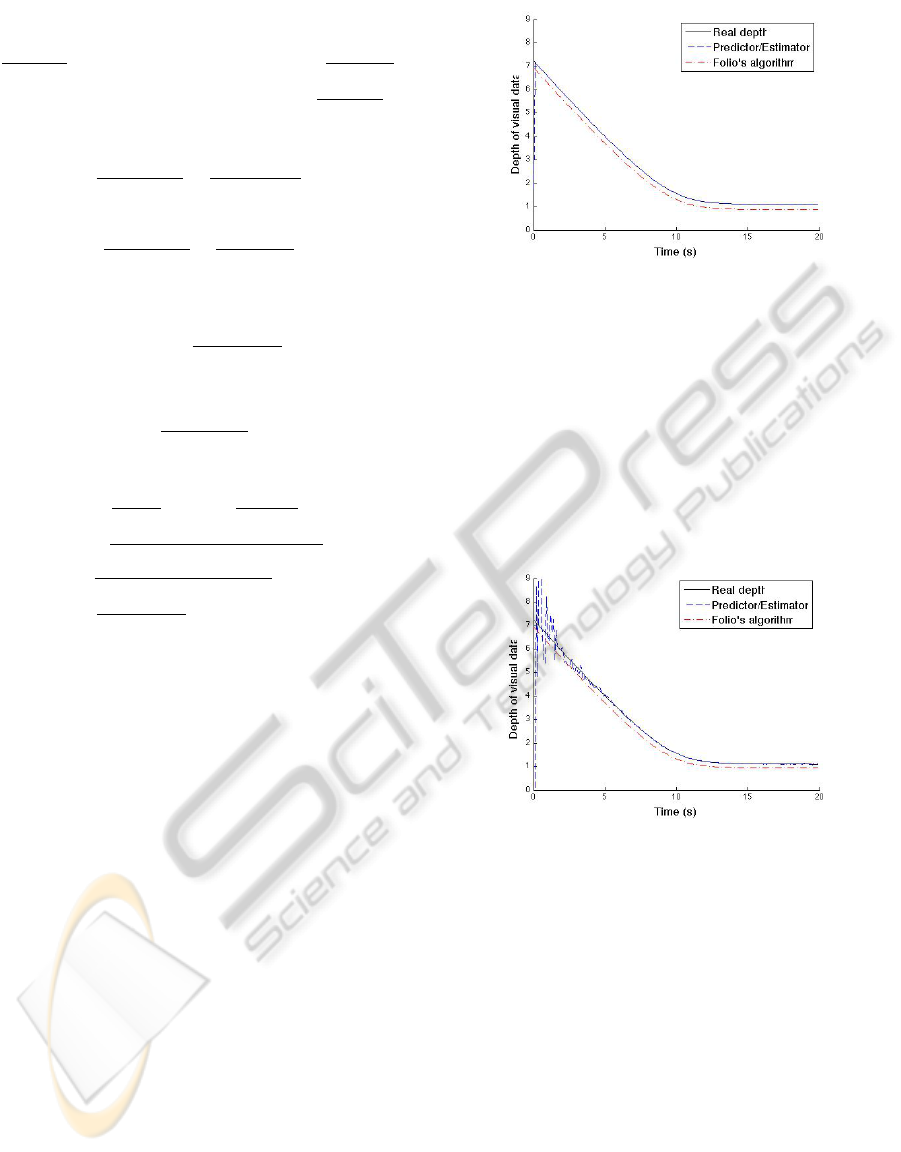
In the first simulation, all the data are supposed to
be perfectly known. As one can see, the obtained esti-
mation of the depth of each point p
i
is perfect, which
validates estimator (21) in the ideal case. Notice that
a good estimated value of depth is immediately ob-
tained, which is not the case of the method proposed
Figure 2: Evolution of both estimated and real depths of one
point P
i
.
in (De Luca et al., 2008). Moreover, we can see the
depth estimation using Folio’s algorithm. The initial
condition is not the real value. The error between
them is preserved during the entire simulation.
Now, we aim at validating estimator (21) when
the visual data are noisy. A one pixel noise has been
added on
˜
X
i
and
˜
Y
i
. In this case the estimator uses at
most m = 20 images. The corresponding results for
one point are represented on figure 3. In a noisy con-
Figure 3: Evolution of both estimated and real depths.
text, estimator (21) converges towards the real depth
value within an acceptable time. Indeed the estimated
depth value is correct after about 2 s. The number of
images m used in the estimation process can be tuned
to fit the performances of the considered testbed. Fi-
nally, to show that our algorithm provides an adequate
value of z sufficiently rapidly, we have coupled it to D.
Folio’s estimation method. Thus, in the same condi-
tions as previously, we have simulated a loss of visual
data between the seventh and ninth seconds during a
visual servoing task. As shown in figure 4, the esti-
mated depth values allow to correctly reconstruct the
visual features. The navigation task can then be cor-
rectly realized, although the controller has been com-
puted with the estimated data instead of the real ones.
This last result demonstrates the efficiency of the pro-
posed approach in a noisy context. D. Folio’s algo-
ICINCO 2010 - 7th International Conference on Informatics in Control, Automation and Robotics
272

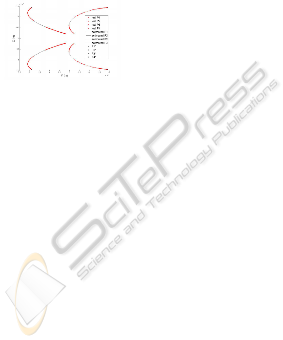
rithm accuracy is then significantly improved thanks
to our approach.
Figure 4: Evolution of estimated and real visual features.
5 CONCLUSIONS
In this paper, we have presented a method allowing
to estimate the depth z
i
during a vision-based navi-
gation task. The proposed approach relies on a pre-
dictor/estimator pair able to provide an estimation of
z
i
, even when the visual data are noisy. The advan-
tage of the proposed approach is that it relies on a
parameterizable number of images, which can be ad-
justed depending on the computation abilities of the
considered processor. The reconstructed depth value
is then used to feed Folio’s algorithm, increasing its
accuracy. The obtained results have proven the ef-
ficiency of our technique in a noisy context. Up to
now, we have only used the estimated value of z
i
to
improve Folio’s work. In the future, we plan to ben-
efit from this value at two different levels. The first
one concerns the control law design with the compu-
tation of L
(s,z)
. The approximations classically made
in the visual servoing area could then be overcome.
The second level is related to the determination of the
reference visual signals s
∗
. This term is computed ei-
ther experimentally by taking an image at the desired
position or theoretically by means of models. These
solutions significantly reduce autonomy. We believe
that a precise estimation of the depth can be very help-
ful to automatically on-line compute the value of s
∗
,
suppressing the above mentioned drawbacks. Finally,
another challenging aspect of our future work will
consist experimenting our approach on a real robot.
REFERENCES
Cervera, E., Martinet, P., and Berry, F. (2002). Robotic
manipulation with stereo visual servoing. Robotics
and Machine Perception, SPIE International Group
Newsletter, 1(1):3.
Chaumette and Hutchinson (2006). Visual servo control,
part 1 : Basic approaches. IEEE Robotics and Au-
tomation Magazine, 13(4).
Comport, Pressigout, Marchand, and Chaumette (2004).
Une loi de commande robuste aux mesures aberrantes
en asservissement visuel. In Reconnaissance des
Formes et Intelligence Artificielle, Toulouse, France.
Corke, P. (1996). Visual control of robots : High perfor-
mance visual servoing. Research Studies Press LTD.
De Luca, Oriolo, and Giordano (2008). Features depth
observation for image based visual servoing: theory
and experiments. Int. Journal of Robotics Research,
27(10).
Djeridane (2004). Sur la commandabilit
´
e des syst
`
emes non
lin
´
eaires
`
a temps discret. PhD thesis, Universit
´
e Paul
Sabatier - Toulouse III.
Durand Petiteville, A., Courdesses, M., and Cadenat, V.
(2009). Reconstruction of the features depth to im-
prove the execution of a vision-based task. In 9th In-
ternational workshop on Electronics, Control, Mod-
elling, Measurement and Signals 2009, Mondragon,
Spain.
Espiau, Chaumette, and Rives (1992). A new approach to
visual servoing in robotics. IEEE Trans. Robot. Au-
tomat., 8:313–326.
Folio and Cadenat (2008). Computer Vision, chapter 4.
Xiong Zhihui; IN-TECH.
Jerian, C. and Jain, R. (1991). Structure from motion: a
critical analysis of methods. IEEE Transactions on
systems, Man, and Cybernetics, 21(3):572–588.
Ma, Y., Soatto, S., Kosecka, J., and Sastry, S. (2003). An in-
vitation to 3-D vision: from images to geometric mod-
els. New York: Springer-Verlag.
Matthies, Kanade, and Szeliski (1989). Kalman filter-based
algorithms for estimating depth in image sequences.
Int, Journal of Computer Vision, 3(3):209–238.
Pissard-Gibollet and Rives (1995). Applying visual ser-
voing techniques to control a mobile handeye sys-
tem. In IEEE Int., Conf. on Robotics and Automation,
Nagoya, Japan.
Samson, Borgne, and Espiau (1991). Robot control : The
task function approach. Oxford science publications.
A NEW PREDICTOR/CORRECTOR PAIR TO ESTIMATE THE VISUAL FEATURES DEPTH DURING A
VISION-BASED NAVIGATION TASK IN AN UNKNOWN ENVIRONMENT - A Solution for Improving the Visual
Features Reconstruction During an Occlusion
273

APPENDIX
Parameters for equation (11):





















































α
i
=
˜
Y
i
(k−1)
f
sin(A( ˙q(k − 1))T ) + cos(A( ˙q(k − 1))T )
β =
n
−D
x
sin(ϑ(k − 1))−
υ(k−1)
ω(k−1)
cos(ϑ(k − 1))+C
y
o
sin(A( ˙q(k − 1))T )+
n
D
x
cos(ϑ(k − 1))−
υ(k−1)
ω(k−1)
sin(ϑ(k − 1))+C
x
o
cos(A( ˙q(k − 1))T )
−D
x
cos(ϑ(k)) +
υ(k−1)
ω(k−1)
sin(ϑ(k)) −C
x
κ
i
=
n
−
˜
Y
i
(k−1)β
f α
i
− D
x
sin(ϑ(k − 1))−
υ(k−1)
ω(k−1)
cos(ϑ(k − 1))+C
y
o
cos(A( ˙q(k − 1))T )−
n
−β
α
i
+ D
x
cos(ϑ(k − 1))−
υ(k−1)
ω(k−1)
sin(ϑ(k − 1))+C
x
o
sin(A( ˙q(k − 1))T ) + D
x
sin(ϑ(k)) +
υ(k−1)
ω(k−1)
cos(ϑ(k)) −C
y
Parameters for equations (20) and (21):



ϑ( j
0
) = ϑ(k − j)+ ϖ
e1
T
ϑ(k) = ϑ(k − j) +(ϖ
e1
+ ϖ
e2
)T















φ
i
=
˜
Y
i
(k− j)
f
sin(A( ˙q
e1
)T ) + cos(A( ˙q
e1
)T )
ϕ
i
=
n
−D
x
sin(ϑ(k)) −
υ
e1
ϖ
e1
cos(ϑ(k − j)) +C
y
o
sin(A( ˙q
e1
)T )
+
n
D
x
cos(ϑ(k − j)) −
υ
e1
ϖ
e1
sin(ϑ(k − j)) +C
x
o
cos(A( ˙q
e1
)T )
−D
x
cos(ϑ( j
0
)) +
υ
e1
ϖ
e1
sin(ϑ( j
0
)) −C
x















































φ
0
i
=
˜
Y
i
(k− j)
f φ
cos(A( ˙q
e1
)T ) sin(A( ˙q
e2
)T ) −
sin(A( ˙q
e1
)T ) sin(A( ˙q
e2
)T )
φ
+cos(A( ˙q
e2
)T )
ϕ
0
i
=
hn
˜
Y
i
(k− j)ϕ
i
f φ
i
− D
x
sin(ϑ(k − j)) −
υ
e1
ω
e1
cos(ϑ(k − j)) +C
y
)
o
cos(A( ˙q
e1
)T )
−
n
−ϕ
i
φ
i
+ D
x
cos(ϑ(k − j)) −
υ
e1
ω
e1
sin(ϑ(k − j)) +C
x
o
sin(A( ˙q
e1
)T )
+(
υ
e1
ω
e1
−
υ
e2
ω
e2
)cos(ϑ( j
0
))
i
sin(A( ˙q
e2
)T )
+
n
D
x
cos(ϑ( j
0
)) −
υ
e2
ω
e2
sin(ϑ( j
0
)) +C
x
o
cos(A( ˙q
e2
)T )
−D
x
cos(ϑ(k)) −
υ
e2
ω
e2
sin(ϑ(k)) +C
x
(
µ
i
= φ
i
φ
0
i
ν
i
= ϕ
i
φ
0
i
+ ϕ
0
i









































γ
i
=
hn
−
˜
Y
i
(k− j)ν
i
f µ
i
− D
x
sin(ϑ(k − j)) −
υ
e1
ω
e1
cos(ϑ(k − j)) +C
y
o
cos(A( ˙q
e1
)T )
−
n
−ν
i
µ
i
+ D
x
cos(ϑ(k − j)) −
υ
e1
ω
e1
sin(ϑ(k − j)) +C
x
o
sin(A( ˙q
e1
)T )
+(
υ
e1
ω
e1
−
υ
e2
ω
e2
)cos(ϑ( j
0
))
i
cos(A( ˙q
e2
)T )
−

−ϕ
0
i
φ
0
i
+ D
x
cos(ϑ( j
0
)) −
υ
e2
ω
e2
sin(ϑ( j
0
)) +C
x

sin(A( ˙q
e2
)T )
+D
x
sin(ϑ(k)) +
υ
e2
ω
e2
cos(ϑ(k)) −C
y
ICINCO 2010 - 7th International Conference on Informatics in Control, Automation and Robotics
274