3D PATH PLANNING FOR UNMANNED AERIAL VEHICLES USING

VISIBILITY LINE BASED METHOD

Rosli Omar

1,2

and Dawei Gu

Faculty of Electrical and Electronic Engineering, Universiti Tun Hussein Onn Malaysia, Johor, Malaysia

Department of Engineering, University of Leicester, LE1 7RH, Leicester, U.K.

Keywords:

3D path planning, Visibility lines, Base line oriented visibility line, Optimization.

Abstract:

In path planning, visibility graph (or visibility line (VL)) method is capable of producing shortest path from

a starting point to a target point in an environment with polygonal obstacles. However, the run time increases

exponentially as the number of obstacles grows, causing this method ineffective for real-time path planning.

A 2D path planning framework based on VL has recently been introduced to ﬁnd a 2D path in an obstacle-

rich environment with low run time. In this paper we propose 3D path planning algorithms based on the 2D

framework. Several steps are used in the algorithms to ﬁnd a 3D path. First, a local plane is generated from a

local starting point to a target point. The plane is then rotated at several pre-deﬁned angles. At each rotation,

a shortest path is calculated using 2D algorithms. After rotations at all angles have been done, the shortest

one is selected. Simulation results show that the proposed 3D algorithms are capable in ﬁnding paths in 3D

environments and computationally efﬁcient, thus suitable for real time application.

1 INTRODUCTION

Uninhabited Aerial Vehicles (UAVs) are becoming

more popular in accomplishing tasks in adverse en-

vironments. For example UAVs have been used for

military purpose such as reconnaissance and combat

as well as to perform civil tasks such as weather fore-

casting, environmental research, search and rescue

missions and trafﬁc control.

The advantage of UAVs in avoiding human loss

brings ”less” intelligence of the vehicle. In order

to make UAVs more practically useful, it is impor-

tant to raise the autonomy level of UAVs. Autonomy

means the capability of UAVs to make its own de-

cisions based on the available information captured

by sensors, and potentially covers the whole range

of the vehicle operations without human interven-

tion (Frampton, 2008). However, autonomy tech-

nology is still in its early stage and fairly under-

developed (http://www.theuav.com). It is the bottle-

neck for UAVs development in the future. Hence the

problem of autonomy has to be addressed before the

fully autonomous UAVs can be advanced. As path

planning is one of the crucial factors in enhancing the

autonomy level in UAVs, this paper focuses on this

topic.

Researches onpath planning amongpolygonalob-

stacles have been around probably since the beginning

of mobile robot. They have produced many meth-

ods and algorithms under several categories. Among

them are geometric-based (Omar and Gu, 2009; Cole-

man and Wunderlich, 2008; Tian et al., 2007; Bortoff,

2000; Nilsson, 1984), grid-based (Chen et al., 1995;

LingelBach, 2004) and potential ﬁeld (Garibotto and

Masciangelo, 1991; Barraquand et al., 1992), to name

but three. One of the popular methods is geometric-

based category under which there is an approach

called visibility lines (VL).

VL was ﬁrst proposed by Lozano-Perez and Wes-

ley (Lozano-Perez and Wesley, 1979) for path plan-

ning in the environments with polyhedral obstacles.

Since then several researchers (Nilsson, 1984; Huang

and Chung, 2004; Bygi and Ghodsi, 2006) used the

method with some variants. However one major dis-

advantage of VL is the computationaleffort grows ex-

ponentially as the number of obstacles increases. To

overcome such a problem, Huang and Chung (Huang

and Chung, 2004) introduced Dynamic VG (DVG)

which used local region to plan a path to speed up

the run time. The local region was determined by the

nodes that have maximum distance from a line drawn

from starting point to target point called S-G line. In

(Omar and Gu, 2009), we proposed 2D path plan-

ning algorithm which was based on VL called Base-

Omar R. and Gu D. (2010).

3D PATH PLANNING FOR UNMANNED AERIAL VEHICLES USING VISIBILITY LINE BASED METHOD.

In Proceedings of the 7th International Conference on Informatics in Control, Automation and Robotics, pages 80-85

DOI: 10.5220/0002881100800085

 SciTePress

Line Oriented Visibility Lines(BLOVL). Also there is

a sub-algorithm of BLOVL named Core. Core’s main

purpose is to ﬁnd a path from a two-stage process.

First, a group of obstacles that lie on base line (BL)

and their extension are identiﬁed. BL is similar to S-

G line in (Huang and Chung, 2004). Second, a path

is calculated using Dijkstra’s algorithm. As the path

planned by Core might not collision-free, BLOVL is

used to further plan it. In addition BLOVL is designed

to be used for real-time path planning.

On the other hand, 3D path planning problems

have been studied extensively for many years. There

were several different approaches available includ-

ing Evolutionary Algorithms (EA) (Hasircioglu et al.,

2008; Mittal and Deb, 2007), VL (Jiang et al., 1993)

and Dubin circles (Ambrosino et al., 2006), to name

but three. In (Hasircioglu et al., 2008) EA and B-

spline curves for off-line 3D path planning were used.

To increase the performance of the path, the number

of generations had to be increased hence increased

the run-time. Like (Hasircioglu et al., 2008), Mittal

and Deb (Mittal and Deb, 2007) presented an off-line

path planner with multi-objective EA and B-spline.

The results of their work were several optimal 3D

paths. (Ambrosino et al., 2006) used Dubin circles to

ﬁrst obtain estimate of a 3D path. Then the path was

divided into three sub-paths. However, (Ambrosino

et al., 2006) assumed that no obstacle to be avoided

during the path generation.

In this paper, we propose a 3D path planning al-

gorithm, BLOVL

which consists of several sub-

algorithms namely BasePlane, Rotate

as well as

BLOVL. Basically BLOVL

ﬁnd the 3D path from a

series of rotations of local planes. This algorithm and

its sub-algorithms have been realized into a Matlab’s

graphical user interface (GUI) environment for simu-

lation purpose to evaluate its effectiveness. The rest of

this paper is organized as follows. Section 2 reviews

the 2D path planning using Core and BLOVL algo-

rithms. Section 3 explains our proposed 3D path plan-

ning algorithm in details. Section 4 shows an example

of results from the proposed algorithms. In Section 5

we demonstrate the simulation results in term of run

time. Section 6 concludes the paper.

2 2D PATH PLANNING

In order to make path calculation faster by visibility

lines (VL) means, the number of obstacles used in the

calculation has to be minimized. Thus Core has been

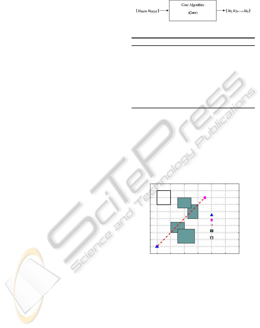
designed to perform this task. Figure 1 illustrates the

process of Core while Algorithm 1 shows the steps

of it.

Figure 1: Core algorithm.

Algorithm 1: Core.

1: Create a base line (BL) from starting point, u

start

to target point, u

target

2: Construct a set of nodes, N

, from the four cor-

ners of each obstacle that lies on the base line and

their extensions, including u

start

and u

target

3: Create a cost matrix, C

from N

4: Find local path, U(u

, . .. , u

) from C

using Di-

jkstra’s algorithm where u

= u

start

and u

target

Core begins with creating a base line (BL) from a

local starting point, u

start

to a target point, u

target

. The

obstacles that lie on BL and their extension, O

will

be used for path calculation. The idea on how O

identiﬁed is illustrated in Figure 2. In the ﬁgure, the

obstacles that intersect with BL arenumberedas 1 and

2 while the extended obstacles are 3 and 4. Obstacle 5

is ignored as it is neither on BL nor an extension of the

obstacles on BL. As a result O

contains obstacles

with the number of 1, 2, 3 and 4.

0 20 40 60 80 100 120

−10

Starting point

Target point

Base line

Included obstacles

Ignored obstacle

Figure 2: Obstacles identiﬁcation using Core.

In Step 2 of Core, O

is used to build up a set

of nodes stored in N

. Then each pair of mutually

visible nodes in N

is connected by a line segment

and given a cost based on its Euclidean distance. On

the contrary, two mutually-invisible nodes are given

inﬁnity costs and are thus ignored. Based on N

, in

the next step of Core, a cost matrix, C

is created.

stores the indexes of paired nodes and the lines

segment Euclidean distances (costs). If all pairs of

mutually-visible nodes are connected together by line

segments, they will form a plane with zero altitude as

shown in Figure 3.

Using C

, Dijkstra’s algorithm will then be ap-

3D PATH PLANNING FOR UNMANNED AERIAL VEHICLES USING VISIBILITY LINE BASED METHOD

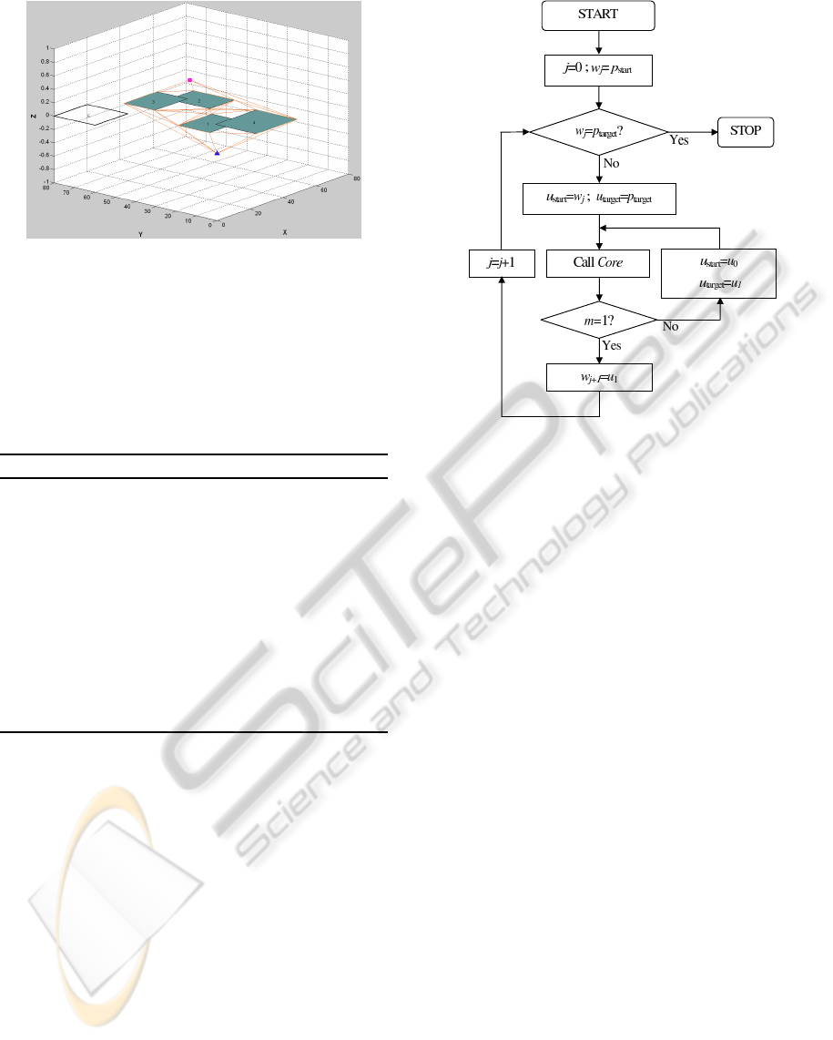
Figure 3: A plane formed by visibility lines with zero alti-

tude.

plied in Step 4 of Core to ﬁnd a local optimal path,

U by minimizing the total path length from u

start

target

. To ensure that the path is collision-free and

capable to be used for real-time path planning, Core

has to be associated with BLOVL as shown in Algo-

rithm 2. Figure 4 shows the BLOVL process.

Algorithm 2: BLOVL.

1: Set j = 0 and w

= p

start

2: while w

6= p

target

3: set u

start

= w

and u

target

= p

target

4: call Core

5: if m = 1 then

6: set w

j+1

= u

7: else

8: set u

target

= u

9: goto line 4

10: end if

11: set j = j + 1

12: end while

The ﬁrst step of BLOVL is setting the current

starting point/waypoint, w

to p

start

where j is ini-

tialized to 0. Then w

is compared with the p

target

If w

is or at the vicinity of p

target

, then the process

is stopped. Otherwise w

and p

target

will be deﬁned

as u

start

and u

target

respectively. With u

start

and u

target

being the input, Core is called to ﬁnd a local shortest

path, U. Core will be called again if the number of el-

ements in U is greater than 2 as this shows that there

are obstacles between u

start

and u

target

. Note that the

element number in U is indicated by m. If m = 1,

it means that U has 2 elements and the resulted path

is unobstructed from u

start

and u

target

, and the next

waypoint w

j+1

will be set to u

. This process will be

repeated until w

is or near to p

target

. Notice that the

resulted path from BLOVL consists of a set of global

waypoints, W = w

, . . . , w

n−1

Figure 4: BLOVL process.

3 ALGORITHM FOR 3D PATH

PLANNING

In practice UAV ﬂies in 3D environments. To en-

sure that the UAV’s paths are free from collision in

such environments, path in 3D has to be planned. For

such a purpose, we have developed 3D path planning

algorithm, BLOVL

which consists of several sub-

algorithms i.e. BasePlane, Rotate

and BLOVL.

BLOVL

uses rotational planes to ﬁnd 3D paths.

Figure 5 illustrates the process of BLOVL

and Al-

gorithm 3 shows its steps.

BLOVL

starts with initializing several neces-

sary parameters i.e. k = 0, Ps

= p

start

and i = 0. No-

tice that Ps is the global path with several waypoints

that will be built-up along the process. The ﬁnal value

of k will determine the number of waypoints in Ps. i

represents the index of the rotational angles.

In the next step of BLOVL

, the vector of rota-

tional angle, α is deﬁned. It consists of b number of

angles. α will determine at which angle the plane will

be rotated. Next Ps

is compared with p

target

. If Ps

is p

target

or at the vicinity of p

target

the process will

be stopped. Otherwise u

start

will be set to Ps

while

target

is p

target

. Note that u

start

and u

target

are nec-

essary for Core of BLOVL in the later stage of the

algorithm.

In case of Ps

is not the p

target

or not at the

vicinity of it, BasePlane which is shown in Algo-

rithm 4 is then called. BasePlane generates a local

plane, Px

′

start

. As shown in Algorithm 4, the local

ICINCO 2010 - 7th International Conference on Informatics in Control, Automation and Robotics

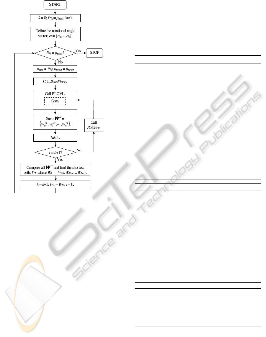
Figure 5: BLOVL

process.

plane generated by BasePlane always change with the

change in u

start

hence it is named Px

′

start

To generate Px

′

start

using BasePlane, ﬁrst a base

line, BL

is drawn from u

start

to u

target

. As u

start

and u

target

have different altitude, the angle β between

and the horizontal global plane, Pxy

start

can be

calculated. BL

⊥

that intersects u

start

and orthogonal

to BL

is then deﬁned. With BL

and BL

⊥

as the

x- and y-axis respectively, Px

′

start

that lies at β de-

gree from Pxy

start

is deﬁned. Then the coordinate of

obstacles lying on Px

′

start

is projected accordingly.

As Px

′

start

has been deﬁned, next is to rotate the

plane by α

degree to ﬁnd a local optimal path, W

αi

from u

start

to u

target

. Rotating this plane is performed

by Rotate

while ﬁnding W

αi

is accomplished by

BLOVL and Core. Algorithm 5 shows Rotate

While i < b + 1, i is increased by 1 and α

updated accordingly and Rotate

and BLOVL are

kept called to ﬁnd W

αi

. When i = b + 1, all paths

(and their costs) that have been stored in W

are

compared with each other and path with the lowest

cost, Ws is then selected. Notice that Ws consists of

{Ws

, . . . ,Ws

n−1

} and the waypoints in Ws are ac-

cording to the global coordinate system.

In the next step, the index of global waypoints, k

is increased by 1 and the next global waypoint, Ps

is updated to be the second waypoint of the shortest

path i.e. Ws

. i then is initialized back to 0 and the

process as described above are repeated until Ps

is or

at the vicinity of p

target

Algorithm 3: BLOVL

1: Set k = 0, Ps

= p

start

and i = 0.

2: Deﬁne the rotational angle vector, α.

3: while Ps

6= p

target

4: u

start

= Ps

; u

start

= p

target

5: call BasePlane to generate local plane,

′

start

6: while i 6= b+ 1 do

7: call BLOVL.

8: Save waypoints, W

generated by BLOVL.

9: Increase i by 1.

10: Rotate Px

′

start

by α

degree.

11: end while

12: Compare all paths in W

and ﬁnd the shortest,

Ws. Ws = {Ws

, . . . ,Ws

13: Increase k by 1 and update Ps

= Ws

. Ini-

tialise i to .

14: end while

Algorithm 4: BasePlane.

1: Draw a base line, BL

connecting u

start

and

target

. Find out the angle β between BL

and the horizontal plane Pxy

start

, which contains

start

2: Deﬁne a local plane, Px

′

start

, formed by BL

and the straight line, BL

⊥

which passes u

start

lies on Pxy

start

and is orthogonal to BL

3: Deﬁne a local coordinate system on Px

′

start

with u

start

as the origin, BL

⊥

as x-axis and BL

as y-axis. Establish the coordinate transforma-

tion between this local coordinate system and the

global one.

4: Project the obstacles on Px

′

start

Algorithm 5: Rotate

1: Rotate the plane Px

′

start

by α

degree.

2: Find out the coordinate transformation between

the new local system and the global one.

3: Project the obstacles on the new Px

′

start

plane.

4 EXAMPLE

A random scenario with 150 obstacles was gener-

ated as shown in Figure 6. Each obstacle was

3D PATH PLANNING FOR UNMANNED AERIAL VEHICLES USING VISIBILITY LINE BASED METHOD

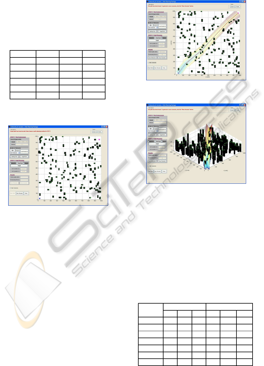
numbered and given a random height. Starting

point’s altitude was set to 20 while the target point’s

altitude was 150. The planes were rotated at

0, 10, 30, 45, 60, 120, 135, 150, 170. The resulted path

had the waypoints as shown in Table 1.

Table 1: The waypoints.

Number X Y Z

1 26.48 18.29 20.00

2 143.76 171.24 41.05

3 394.24 378.76 69.72

4 576.76 581.24 98.77

5 817.76 834.25 133.93

6 959.76 960.92 150.00

Figure 7 and Figure 8 show the top and 3D views

of the resulted path respectively.

Figure 6: A random scenario with obstacles shown in black.

The blue rectangle is the starting point and the square ma-

genta is the target point.

5 SIMULATION RESULTS

Scenarios with several numbers of obstacles were

simulated randomly to evaluate the performance of

the proposed 3D path planning algorithms. The num-

ber of obstacles used were 50, 75, 100, 125, 150, 175

and 200. To increase the reliability of the results,

ten different random scenarios were generated from

each number of obstacles. The simulations were per-

formed on Intel’s 2.4Ghz Core 2 Duo processor with

2GB DDR2 RAM. As no data for other 3D algorithms

available in the literature using the same scenarios as

we used here, no comparison was done. Thus we

compared the proposed 3D path planning algorithm

performance with that of 2D that was introduced by

(Omar and Gu, 2009) as both algorithms were de-

signed for such scenarios. The results of the simu-

lation were recorded in Table 2.

Figure 7: Top view of the resulted path (in red) with the

rotated planes.

Figure 8: 3D view of the resulted path with the rotated

planes.

From Table 2, using 2D algorithms no substantial

growth in run time as the number of obstacles were in-

creased while by 3D algorithms the calculation time

increased quite signiﬁcantly. This is due to (i) in-

creased number of obstacles on the base line which

results in increased number of waypoints. (ii) number

of angles used to generate the rotational planes. If the

resulted path has k waypoints and the rotational angle

vector, α consists of b number of angles, the process-

ing time might be (b − 1) × k longer than that of 2D

path planning algorithms.

Table 2: Comparison of 2D and 3D path planning algo-

rithms performance (in sec).

Number of 2D Algorithms 3D Algorithms

obstacles Min Max Ave Min Max Ave

50 0.01 0.25 0.13 0.65 1.84 1.27

75 0.02 0.20 0.15 1.03 6.93 2.63

100 0.04 0.28 0.21 1.97 8.14 4.08

125 0.06 0.39 0.27 2.59 17.54 8.77

150 0.08 0.43 0.35 5.18 22.16 11.63

175 0.15 0.83 0.50 6.82 35.79 21.13

200 0.19 0.98 0.62 7.16 48.77 26.42

ICINCO 2010 - 7th International Conference on Informatics in Control, Automation and Robotics

6 CONCLUSIONS

As visibility line (VL) method is effective in produc-

ing path with shortest length, it has been used to de-

velop a three-dimensional (3D) path planning algo-

rithm, BLOVL

. BLOVL

governsBasePlane, Ro-

tate

as well as Base Line Oriented Visibility Line

(BLOVL) algorithms to ﬁnd a 3D path. BasePlane

algorithm is used to establish a local plane. Next Ro-

tate

algorithm rotates the plane. At each rotation

of the plane, a path with lowest cost is calculated by

BLOVL and recorded. After the local plane has been

rotated at all angles, the resulted paths are compared

to each other and the shortest one will be selected.

The process continues with a newstarting point which

is the second waypoint of the previous shortest path.

The process is stopped if the target point has been

reached. Simulations results show that BLOVL

and

its sub-algorithms are capable to effectively ﬁnd sub-

optimal paths in term of path length in 3D environ-

ments and is very promising to be applied in real time

3D path planning.

REFERENCES

Ambrosino, G., Ariola, M., Ciniglio, U., Corraro, F.,

Pironti, A., and Virgilio, M. (2006). Algorithms for

3d uav path generation and tracking. In Proceedings

of the 45th IEEE Conference on Decision and Control,

pages 5275–5280. IEEE.

Barraquand, J., Langlois, B., and Latombe, J.-C. (1992).

Numerical potential ﬁeld techniques for robot path

planning. In Proceedings of the IEEE Transactions on

Systems, Man and Cybernetics, pages 224–240. IEEE.

Bortoff, S. (2000). Path planning for uavs. In Proceedings

of the American Control Conference Chicago Illinois,

pages 364–368. ACC.

Bygi, M. and Ghodsi, M. (2006). 3d visibility graph. In 12th

CSI Computer Conference (CSICC 2006). Computer

Society of Iran.

Chen, D., Szczerba, R., and Uhran, J. (1995). Planning con-

ditional shortest paths through an unknown environ-

ment: A framed-quadtree approach. In Proceedings

of the International Conference on Intelligent Robots

and Systems, pages 33–38. IEEE.

Coleman, D. and Wunderlich, J. (2008). O3: An optimal

and opportunistic path planner (with obstacle avoid-

ance) using voronoi polygons. In International Work-

shop on Advanced Motion Control, pages 371–376.

IEEE.

Frampton, R. (2008). Uav autonomy. The Journal for De-

fence Engineering & Science, 1(Summer 2008):28–

31.

Garibotto, G. and Masciangelo, S. (1991). Path planning

using the potential ﬁeld approach for navigation. In

Fifth International Conference on Advanced Robotics.

IEEE.

Hasircioglu, I., Topcuoglu, H., and Ermis, M. (2008). 3-d

path planning for the navigation of unmanned aerial

vehicles by using evolutionary algorithms. In Pro-

ceedings of the 10th Annual Conference on Genetic

and Evolutionary Computation, pages 1499–1506.

ACM.

Huang, H. and Chung, S. (2004). Dynamic visibility graph

for path planning. In Proceeding of International Con-

ference on Intelligent Robots and Systems. IEEE.

Jiang, K., Seneviratne, L., and Earles, S. (1993). Finding the

3d shortest path with visibility graph and minimum

potential energy. In Proceeding of the 1993 IEEE/RSJ

International Conference on Intelligent Robots and

Systems, pages 679–684. IEEE.

LingelBach, F. (2004). Path planning using probabilistic

cell decomposition. In Proceedings of the IEEE In-

ternational Conference on Robotics and Automation,

pages 467–472. IEEE.

Lozano-Perez, T. and Wesley, M. (1979). An algorithm for

planning collision-free paths among polyhedral obsta-

cles. In Contmum ACM, pages 560–570. ACM.

Mittal, S. and Deb, K. (2007). Three-dimensional of-

ﬂine path planning for uavs using multiobjective evo-

lutionary algorithms. In Proceedings of the IEEE

Congress on Evolutionary Computation, pages 3195–

3202. IEEE.

Nilsson, N. (1984). Shakey the robot. Technical Report

JReport 323, 333 Ravenswood Avenue, Menlo Park,

CA 94025-3493.

Omar, R. and Gu, D.-W. (2009). Visibility line based meth-

ods for uav path planning. In ICROS-SICE Interna-

tional Joint Conference. ICROS-SICE.

Tian, Y., Yan, L., Park, G., S.Yang, Kim, Y., Lee, S.,

and Lee, C. (2007). Application of rrt-based local

path planning algorithm in unknown environment. In

Proceeding of the IEEE International Symposium on

Computational Intelligence in Robotics and Automa-

tion, pages 456–460. IEEE.

3D PATH PLANNING FOR UNMANNED AERIAL VEHICLES USING VISIBILITY LINE BASED METHOD