IMPROVED MULTISTAGE LEARNING

FOR MULTIBODY MOTION SEGMENTATION

Yasuyuki Sugaya

Department of Computer Science and Engineering, Toyohashi University of Technology, Toyohashi, Aichi 441-8580, Japan

Kenichi Kanatani

Department of Computer Science, Okayama University, Okayama 700-8530, Japan

Keywords:

Multibody motion segmentation, GCAP, Taubin method, EM algorithm, Multistage optimization.

Abstract:

We present an improved version of the MSL method of Sugaya and Kanatani for multibody motion segmen-

tation. We replace their initial segmentation based on heuristic clustering by an analytical computation based

on GPCA, ﬁtting two 2-D afﬁne spaces in 3-D by the Taubin method. This initial segmentation alone can

segment most of the motions in natural scenes fairly correctly, and the result is successively optimized by the

EM algorithm in 3-D, 5-D, and 7-D. Using simulated and real videos, we demonstrate that our method out-

performs the previous MSL and other existing methods. We also illustrate its mechanism by our visualization

technique.

1 INTRODUCTION

Separating independently moving objects in a video

stream has attracted attention of many researchers in

the last decade, and today we are witnessing a new

surge of interest in this problem. The most classical

work is by Costeira and Kanade (1998), who showed

that, under afﬁne camera modeling, trajectories of im-

age points in the same motion belong to a common

subspace of a high-dimensional space. They seg-

mented trajectories into different subspaces by zero-

nonzero thresholding of the elements of the “interac-

tion matrix” computed in relation to the “factorization

method” for afﬁne structure from motion (Poelman

and Kanade, 1997; Tomasi and Kanade, 1992). Since

then, various modiﬁcations and extensions have been

proposed. Gear (1998) used the reduced row eche-

lon form and graph matching. Ichimura (1999) used

the Otsu discrimination criterion. He also used the

QR decomposition (Ichimura, 2000). Inoue and Ura-

hama (2001) introduced fuzzy clustering. Kanatani

(2001, 2002, 2002a) combined the geometric AIC

(kaike Information Criterion) (Kanatani, 1996) and

robust clustering. Wu et al. (2001) introduced orthog-

onal subspace decomposition. Sugaya and Kanatani

(2004) proposed a multistage learning strategy using

multiple models. Vidal et al. (2005, 2008) applied

their GPCA (Generalized Principal Component Anal-

ysis), which ﬁts a high-degree polynomial to multiple

subspaces. Fan et al. (2006) and Yan and Pollefeys

(2006) introduced new voting schemes for classifying

points into different subspaces in high dimensions.

Schindler et al. (2008) and Rao et al. (2008) incorpo-

rated model selection based on the MDL (Minimum

Description Length) principle.

At present, it is difﬁcult to say which is the best

among all these methods. Their performance has been

tested, using real videos, but the result depends on the

test videos and the type of the motion that is taking

place (planar, translational, rotational, etc.). If such

distinctions are disregarded and simply the gross cor-

rect classiﬁcation ratio is measured using a particular

database, typically the Hopkins155 (Tron and Vial,

2007), all the methods exhibit more or less similar

performance.

A common view behind existing methods seems

to be that the problem is intricate because the seg-

mentation takes place in a high-dimensional space,

which is difﬁcult to visualize. This way of thinking

has lead to introducing sophisticated mathematics one

after another and simply testing the performance us-

ing the Hopkins155 database. In this paper, we show

that the problem is not difﬁcult at all and that the ba-

sis of segmentation lies in low dimensions. Indeed,

199

Sugaya Y. and Kanatani K. (2010).

IMPROVED MULTISTAGE LEARNING FOR MULTIBODY MOTION SEGMENTATION.

In Proceedings of the International Conference on Computer Vision Theory and Applications, pages 199-206

DOI: 10.5220/0002814601990206

 SciTePress

we can visualize what is going on in 3-D. This re-

veals that what is crucial is the type of motion and

that different motions can be easily segmented if the

motion type is known.

Sugaya and Kanatani (2004) assumed multiple

candidate motion types and presented the MSL (Mul-

tiStage Learning) strategy, which does not require

identiﬁcation of the motion type. To do this, they

exploited the hierarchy of motions (e.g., translations

are included in afﬁne motions) and applied the EM

algorithm by progressively assuming motion models

from particular to general: Once one tested motion

type agrees with the true one, the segmentation is un-

changed in the subsequent stages because general mo-

tions include particular ones. Tron and Vidal (2007)

did extensive comparative experiments and reported

that MSL is highly effective. In this paper, we present

an improved version of MSL.

Since MSL uses the EM algorithm, we need to

provide an appropriate initial segmentation, which is

the key to the performance of the subsequent stages,

in which the segmentation in the preceding stage is

input and the output is sent to the next stage. For com-

puting the initial segmentation, MSL used a rather

heuristic clustering that combines the interaction ma-

trix of Costeira and Kanade (1998) and model selec-

tion using the geometric AIC (Kanatani, 1996). In

this paper, we replace this by the GPCA of Vidal et

al. (2005, 2008): we ﬁt a degenerate quadric in 3-D

by the method of Taubin (1991). Then, we succes-

sively apply the EM algorithm and demonstrate, us-

ing the Hopkins155 database, that our method out-

performs MSL and other existing methods. We also

show, using our visualization technique, why and how

good segmentation results.

2 AFFINE CAMERAS

Suppose N feature points {p

}are tracked overM im-

age frames. Let (x

κα

), κ = 1, ..., M, be the image

coordinates of the αth point p

in the κth frame. We

call the 2M-D vector

= (x

1α

, y

1α

, x

2α

, y

2α

, ··· x

Mα

, y

Mα

)

⊤

, (1)

the trajectory of p

. Thus, an image motion of each

point is identiﬁed with a point in 2M-D. We deﬁne

a camera-based XYZ coordinate system such that the

Z-axis coincides with the camera optical axis and re-

gard the scene as moving relative to a stationary cam-

era. We also deﬁne a coordinate system ﬁxed to each

of the moving objects. Let (a

) be the coordi-

nates of point p

with respect to the coordinate sys-

tem of the object it belongs to. Let t

be the origin of

that coordinate system and {i

} the basis vec-

tors in the κth frame. Then, the 3-D position r

κα

the point p

in the κth frame with respect to the cam-

era coordinate system is

κα

= t

+ a

+ b

+ c

. (2)

The afﬁne camera, which generalizes ortho-

graphic, weak perspective, and paraperspective pro-

jections (Poelman and Kanade, 1997), models the

camera imaging by



κα



= A

κα

+ b

, (3)

where the 2 ×2 matrix A

and the 2-D vector b

are

determined by the intrinsic and extrinsic camera pa-

rameters of the κth frame. By substitution of Eq. (2),

Eq. (3) is written in the form



κα



0κ

+ a

1κ

+ b

2κ

+ c

3κ

, (4)

where

0κ

1κ

2κ

, and

3κ

are 2-D vectors de-

termined by the intrinsic and extrinsic camera param-

eters of the κth frame. The trajectory in Eq. (1) is

expressed as the vertical concatenation of Eq. (4) for

κ = 1, ..., M, in the form

= m

+ a

+ b

+ c

, (5)

where m

, i = 0, 1, 2, 3, are the 2M-D vectors consist-

ing of

iκ

for κ = 1, ..., M.

3 GEOMETRIC CONSTRAINTS

Equation (5) states that the trajectories of points that

belong to the same object are in a common “4-D

subspace” spanned by {m

, m

}. Hence,

segmenting trajectories into different motions can be

done by classifying them into different 4-D subspaces

in 2M-D. However, the coefﬁcient of m

in Eq. (5)

is identically 1, which means that the trajectories of

points that belong to the same object are in a common

“3-D afﬁne space” passing through m

and spanned

by {m

, m

}. Thus, segmentation can also

be done by classifying trajectories into different 3-D

afﬁne spaces in 2M-D.

In real situations, however, objects and a back-

ground often translate with rotations only around an

axis vertical to the image plane. We say such a mo-

tion is planar; translations in the depth direction can

take place, but they are invisible under the afﬁne cam-

era modeling, so we can regard translations as con-

strained to be in the XY plane. It follows that if we

take the basis vector k

in Eq. (2) to be in the Z di-

rection, it is invisible to the camera, and hence m

VISAPP 2010 - International Conference on Computer Vision Theory and Applications

200

m’

(a) (b)

Figure 1: (a) If the motions are planar, object and back-

ground trajectories belong to different 2-D afﬁne spaces. (b)

If the motions are translational, object and background tra-

jectories belong to 2-D afﬁne spaces that are parallel to each

other.

0 in Eq. (5). Thus, the trajectories of points under-

going the same motion are in a common “2-D afﬁne

space” passing through m

and spanned by {m

, m

}

(Fig. 1(a))

If, moreover, objects and a background merely

translate without rotation, we can ﬁx the basis vectors

and j

in the X and Y directions, respectively. This

means that the vectors m

and m

in Eq. (5) are com-

mon to all the objects and the background. Thus, the

2-D afﬁne spaces are parallelto each other (Fig. 1(b)).

It is well known that the interaction-matrix-based

method of Costeira and Kanade (1998) fails if the mo-

tion is planar. Furthermore, if there exist two 2-D

afﬁne spaces parallel to each other, they are both con-

tained in some 3-D afﬁne space, and hence in some

4-D subspace. This means classiﬁcation of different

motions into 3-D afﬁne spaces or into 4-D subspaces

is impossible. Yet, this type of degeneracy is very fre-

quent in real situations. In fact, almost all “natural”

scenes in the Hopkins155 database undergo such de-

generacy to some extent

. This may be the main rea-

son that many researchers have regarded multibody

motion segmentation as difﬁcult and tried various so-

phisticated mathematics one after another.

The MSL of Sugaya and Kanatani (2004) resolved

this by starting from the translational motion assump-

tion and progressivelyapplying more general assump-

tions so that any degeneracy is not untested. In this

paper, we improve their method by introducing new

analytical initial segmentation and going on to suc-

cessive upgrading in slightly different dimensions.

4 DIMENSION COMPRESSION

In the following, we concentrate on two motions: an

object is moving relative to a background, which is

The exceptions are the artiﬁcial “box” scenes, in which

boxes autonomously undergo unnatural 3-D translations

and rotations. For these, segmentation is very easy.

also moving. If the two motions are both general, the

observed trajectories belong to two 3-D afﬁne spaces

in 2M-D. There exists a 7-D afﬁne space that contains

both. Hence, segmentation of trajectories can be done

in a 7-D afﬁne space: noise components in the out-

ward directions do not affect the segmentation. If we

translate the 7-D afﬁne space so that it passes through

the origin, take seven basis vectors in it, and express

all the trajectories in their linear combinations, each

trajectory can be identiﬁed with a point in 7-D. Simi-

larly, if the observed trajectories are in two 2-D afﬁne

spaces in 2M-D, there exists a 5-D afﬁne space that

contains both. Then, each trajectory can be identiﬁed

with a point in 5-D. If, moreover, the two 2-D afﬁne

spaces in 2M-D are parallel to each other, there exists

a 3-D afﬁne space that contains both, and each trajec-

tory can be identiﬁed with a point in 3-D.

A trajectory in 2M-D can be identiﬁed with a point

in d-D by the following PCA (Principal Component

Analysis):

1. Compute the centroid p

of all the trajectories

} and the deviations

from it:

∑

α=1

= p

−p

. (6)

2. Compute the SVD (Singular Value Decomposi-

tion) of the following 2M×N matrix in the form



, ...,



= Udiag(σ

, ..., σ

⊤

, (7)

where r = min(2M, N), and U and V are 2M ×r

and N × r matrices, respectively, having r or-

thonormal columns.

3. Let u

be the ith column of U, and compute the

following d-D vectors r

, α = 1, ..., N:



(

), ..., (

)



⊤

. (8)

In this paper, we denote the inner product of vectors

a and b by (a,b).

5 INITIAL SEGMENTATION

Now, we describe our analytical initial segmentation

that replaces the heuristic clustering of MSL. We

identify trajectories with points in 3-D by the above

procedure and ﬁt two planes (= 2-D afﬁne spaces).

If the object and the background are both in transla-

tional motions, all the 3-D points belong to two paral-

lel planes. This may not hold if the data are noisy or

rotational components exist, but if the noise is small

and the motions are nearly translational, which is the

IMPROVED MULTISTAGE LEARNING FOR MULTIBODY MOTION SEGMENTATION

201

case in most natural scenes, we can expect that two

planes can ﬁt to all the points fairly well.

A plane Ax+By+Cz+D = 0 in 3-D can be written

as (n,x) = 0, where we put

n = (A, B, C, D)

⊤

, x = (x, y, z, 1)

⊤

. (9)

Two planes (n

,x) = 0 and (n

,x) = 0 can be com-

bined into one in the form

,x)(n

,x) = (x,n

⊤

x) = (x,Qx) = 0, (10)

where we deﬁne the following symmetric matrix Q:

Q =

⊤

+ n

⊤

. (11)

Note that it is a symmetric matrix that deﬁnes a

quadratic form. Equation (11) implies that Q has rank

2 with two multiple zero eigenvalues and that the re-

maining eigenvalues have different signs. Let these

eigenvalues be λ

, 0, 0, −λ

in descending order, and

, u

the corresponding unit eigenvectors.

Then, Q has the following spectral decomposition:

Q=λ

⊤

−λ

⊤





−



⊤



−





⊤

. (12)

Comparing this with Eq. (11) and noting that vectors

and n

(hence the matrix Q) have scale indeter-

minacy, we can determine n

and n

up to scale as

follows:

, n

−

. (13)

Let x

, ..., x

be the 3-D points that represent trajec-

tories. In the presence of noise or rotational compo-

nents, they may not exactly satisfy Eq. (10), so we ﬁt

a quadratic surface (x, Qx) = 0 to them in such a way

that

,Qx

) ≈ 0, α = 1, ...,N. (14)

Once such a Q is obtained (the computation is de-

scribed in the next section), we can determine the

vectors n

and n

that specify the two planes by

Eqs. (13). The distance d of a point (x,y,z) to a plane

Ax+ By +Cz+ D = 0 is

d =

|Ax+ By +Cz+ D|

√

+ B

. (15)

For each point x

, we compute the distances to the

two planes and classify it to the nearer one. The re-

sulting segmentation is fed to the subsequent learning.

The above computation is a special application of

the GPCA of Vidal et al. (2005, 2008), which ex-

presses multiple subspaces as one high-dimensional

polynomial and classiﬁes points into different sub-

spaces by ﬁtting the high-dimensional polynomial to

all the points. Here, we classify points into two afﬁne

spaces using the same principle.

6 HYPERSURFACE FITTING

The matrix Q that satisﬁes Eq. (14) is computed as

follows. In terms of the homogeneous coordinate

vector x deﬁned in Eqs. (9), the equation (x, Qx) =

0 for a symmetric matrix Q deﬁnes a quadric sur-

face, describing an ellipsoid, a hyperboloid, an ellip-

tic/hyperbolic paraboloid, or their degeneracy includ-

ing a pair of planes. We ﬁt a surface (x,Qx) = 0 to the

points x

in 3-D in the same way as we ﬁt a conic (an

ellipse, a hyperbola, a parabola, or their degeneracy)

to points in 2-D (Kanatani and Sugaya, 2007). If we

deﬁne 9-D vectors z

and u by

=(x

,2y

,2z

,2x

,2y

,2z

)

⊤

v= (Q

)

⊤

, (16)

Eq. (14) is rewritten as

,v) + Q

≈ 0, α = 1,...,N. (17)

A well known method for computing such v and

is the method of Taubin (1991), which is known

to be highly accurate as compared with naive least

squares (Kanatani, 2008; Kanatani and Sugaya 2007).

Theoretically, ML (Maximum Likelihood) achieves

higher accuracy (Kanatani, 2008; Kanatani and Sug-

aya, 2007), but the surface (x,Qx) = 0 that degener-

ates into two planes has singularities along their inter-

section. We have observed that iterations for ML fail

to converge when some data points are near the singu-

larities; the corresponding denominators diverge and

become ∞ if they coincide with singularities

The Taubin method in this case goes as follows.

Assume that x

, y

, and z

are perturbed by Gaussian

noise ∆x

, ∆y

, and ∆z

, respectively, of mean 0 and

standard deviation σ. Let ∆z

be the perturbation of

in Eqs. (16). By ﬁrst order expansion, we have

∆z

=(2x

∆x

,2y

∆y

,2z

∆z

,2∆y

+ 2y

∆z

..., 2∆z

)

⊤

, (18)

from which we can evaluate the covariance matrix

V[z

] = E[∆z

∆z

⊤

] of z

. Noting the relations E[∆x

]

= E[∆y

] = E[∆z

] = 0, E[∆y

∆z

] = E[∆z

∆x

] =

E[∆x

∆y

] = 0, and E[∆x

] = E[∆y

] = E[∆z

] = σ

we obtain V[z

] = σ

], where

] =







0 0 0 z

0 0

∗ y

0 y

0 x

0 y

∗ ∗ z

0 0 0 z

∗ ∗ ∗ y

+ z

0 z

∗ ∗ ∗ ∗ z

+ x

0 x

∗ ∗ ∗ ∗ ∗ x

+ y

∗ ∗ ∗ ∗ ∗ ∗ 1 0 0

∗ ∗ ∗ ∗ ∗ ∗ ∗ 1 0

∗ ∗ ∗ ∗ ∗ ∗ ∗ ∗ 1







. (19)

ML minimizes the sum of the distances, measured in

the direction of the surface normals, to the surface, but no

surface normals can be deﬁned at singularities.

VISAPP 2010 - International Conference on Computer Vision Theory and Applications

202

Here, ∗ means copying the element in the sym-

metric position. The Taubin method minimizes

∑

α=1



,v) + Q



∑

α=1

(v,V

]v)

. (20)

If the denominator is omitted, this becomes the naive

least squares, but the existence of the denominator is

crucial for improving the accuracy as we show later.

The solution {v, Q

} that minimizes Eq. (20) is ob-

tained as follows (Kanatani and Sugaya, 2007):

1. Compute the centroid z

of {z

} and the devia-

tions

from it:

∑

α=1

= z

−z

. (21)

2. Compute the following 9×9 matrices:

∑

α=1

⊤

, N

∑

α=1

]. (22)

3. Solve the generalized eigenvalue problem

v = λN

v, (23)

and compute the unit generalized eigenvector v

for the smallest generalized eigenvalue λ.

4. Compute Q

as follows:

= −(z

,v). (24)

7 MULTISTAGE LEARNING

After an initial segmentation is obtained, we ﬁt afﬁne

spaces by the EM algorithm in successively higher di-

mensions:

1. Two parallel panes in 3-D.

2. Two 2-D afﬁne spaces in 5-D.

3. Two 3-D afﬁne spaces in 7-D.

If the object and the background are in transla-

tional motions, an optimal solution is obtained in the

ﬁrst stage, and it is still optimal in the second and the

third stages. If the object and the backgroundundergo

planar motions with rotations, an optimal solution is

obtained in the second stage, and it is still optimal in

the third. If the object and the background are in gen-

eral 3-D motions, an optimal solution is obtained in

the third stage. Because a degenerate motion is a spe-

cial case of general motions, an optimal solution for

a degenerate motion is unchanged when optimized by

assuming a more general motion. This is the basic

principle of MSL of Sugaya and Kanatani (2004).

The EM algorithm for classifying n-D points r

α = 1, ..., N, into two d-D afﬁne spaces (n ≥ 2d + 1)

is as follows:

1. Using the initial classiﬁcation, deﬁne the mem-

bership weight W

(k)

of r

to class k (= 1, 2) as

follows

(k)



1 if r

belongs to class k

0 otherwise

. (25)

2. For each class k (= 1, 2), do the following compu-

tation:

(a) Compute the prior w

(k)

of class k as follows.

(k)

∑

α=1

(k)

. (26)

(b) If w

(k)

≤ d/N, stop (the number of points is too

small to span a d-D afﬁne space).

(k)

of class k:

(k)

∑

α=1

(k)

∑

α=1

(k)

. (27)

(d) Compute the moment M

(k)

of class k:

(k)

∑

α=1

(k)

−r

(k)

)(r

−r

(k)

)

⊤

∑

α=1

(k)

(28)

Let λ

(k)

≥ ··· ≥ λ

(k)

be the n eigenvalues of

(k)

, and u

(k)

, ..., u

(k)

the corresponding unit

eigenvectors.

(e) Compute the “inward” projection matrix P

(k)

onto class k and the “outward” projection ma-

trix P

(k)

⊥

onto the space orthogonal to it by

(k)

∑

i=1

(k)

(k)⊤

, P

(k)

⊥

= I−P

(k)

. (29)

3. Estimate the square noise level σ

from the square

sum of the “outward” noise components in the

form

=min[

(n−d)(N −d −1)

tr(w

(1)

⊥

(1)

⊥

(2)

⊥

(2)

⊥

),σ

min

], (30)

where tr denotes the trace, and σ

min

is a small

number, say 0.1 pixels, to prevent

from becom-

ing exactly 0, which would cause computational

failure in the subsequent computation, The num-

ber (n −d)(N −d −1) accounts for the degree of

freedom of the χ

-distribution of the square sum

of the “outward” noise components (Kanatani,

1996).

IMPROVED MULTISTAGE LEARNING FOR MULTIBODY MOTION SEGMENTATION

203

4. Compute the covariance matrix V

(k)

of class k (=

1, 2) as follows:

(k)

= P

(k)

⊥

. (31)

The ﬁrst term on the right-hand side is for the data

variations within the afﬁne space; the second ac-

counts for the “outward” noise components.

5. Do the following computation for each point r

α = 1, ..., N:

(a) Compute the conditional likelihood P(α|k), k =

1, 2, of r

P(α|k) =

−(r

−r

(k)

(k)−1

−r

(k)

))/2

√

detV

(k)

. (32)

(b) Update the membership weight W

(k)

, k = 1, 2,

of r

as follows:

(k)

P(α|k)

(1)

P(α|1) + w

(2)

P(α|2)

. (33)

6. Go back to Step 2 and iterate the computation un-

til {W

(k)

} converges.

7. After convergence (or interruption), classify each

to the class k for which W

(k)

, k = 1, 2, is larger.

If we let n = 5 and d = 2, the above procedure is

the second stage of the multistage learning, and if we

let n = 7 and d = 3, it is the third stage. The ﬁrst stage

requires an additional constraint that the two planes be

parallel. For this, we let n = 3 and d = 2 and compute

from the two matrices M

(k)

, k = 1, 2, their weighted

average

M = w

(1)

+ w

(2)

. (34)

Let λ

≥ ··· ≥ λ

be its n eigenvalues, and u

, ...,

the corresponding unit eigenvectors. We let the

projection matrices P

(k)

and P

(k)

⊥

coincide in the form

(1)

= P

(2)

= P and P

(1)

⊥

= P

(2)

⊥

= P

⊥

, where

P =

∑

i=1

⊤

, P

⊥

= I−P. (35)

The estimation of the square noise level σ

in Step 3

is replaced by

= min[

(n−d)(N −d −2)

tr(P

⊥

),σ

min

(36)

The rest is unchanged.

However, there is an inherent problem in EM-

based learning: If there is no noise, its distribution

cannot be stably estimated. This causes no problem

in real situations but may result in computational fail-

ure when ideal data are used for a testing purpose.

(a)

2 4 6 8 10

2 3

(b)

2 4 6 8 10

(c)

2 4 6 8 10

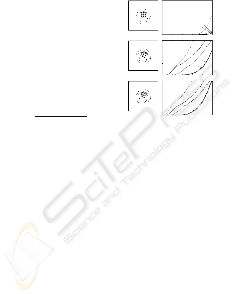
Figure 2: Left column: 20 background points and 14 ob-

ject points. (a) Translational motion. (b) Planar motion. (c)

General 3-D motion. Right column: Average misclassiﬁ-

cation ratio over 5000 trials. The horizontal axis is for the

standard deviation σ of added noise. 0) Initial segmentation

by the Taubin method. 1) Parallel plane ﬁtting in 3-D. 2)

2-D afﬁne space ﬁtting in 5-D. 3) 3-D afﬁne space ﬁtting in

7-D. The dotted lines are for initial segmentation by least

squares.

This phenomenon was reported by Tron and Vidal

(2007) for MSL. In the above procedure, this occurs

when points are exactly in a 2-D afﬁne space in 7-D,

in which case the covariance matrix degenerates to

have rank 2 and hence the likelihood cannot be de-

ﬁned: To deﬁne P(α|k), the matrix V

(k)

in Eq. (31)

must have rank n, and detV

(k)

in the denominator of

Eq. (32) must be positive. To cope with this, our sys-

tem checks if such a degeneracy exists by using the

geometric AIC (Kanatani, 1996), and if so judged, the

3-D afﬁne space is replaced by a 2-D afﬁne space (we

omit the details). Such a treatment does not affect the

performance when real data are used.

8 EXPERIMENTS

8.1 Simulation

The left column of Fig. 2 shows simulated 512×512-

pixel images of 14 object points and 20 background

points in (a) translational motion, (b) planar motion,

and (c) general 3-D motion. These are the 5th of 10

frames; the curves in them are trajectories over the

VISAPP 2010 - International Conference on Computer Vision Theory and Applications

204

(a) (b) (c)

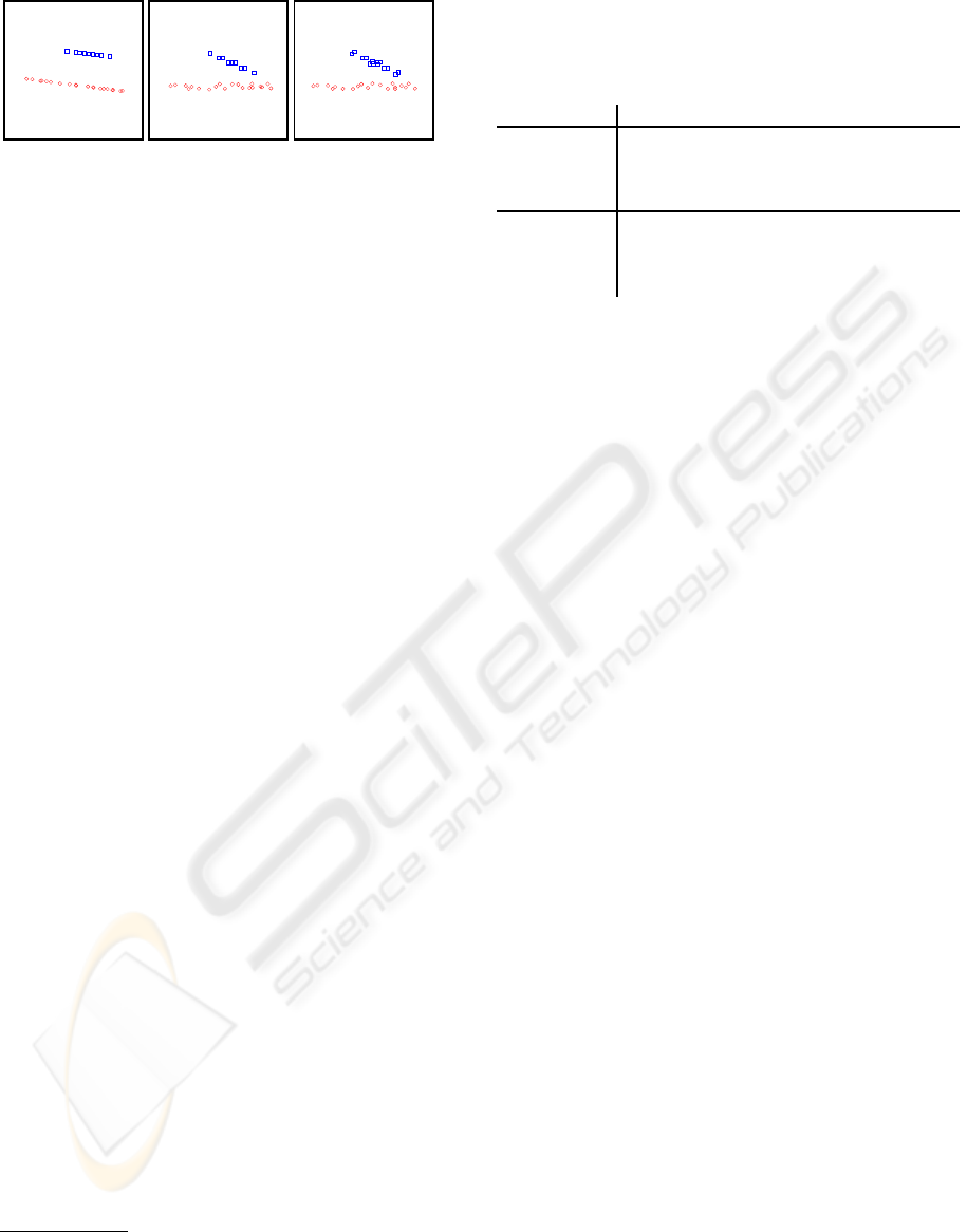
Figure 3: 3-D visualization of image motions in Fig. 2.

10 frames. We added Gaussian noise of mean 0 and

standard deviation σ to the x and y coordinates of each

point in each frame independently, and evaluated the

average misclassiﬁcation ratio over 5000 independent

trials for each σ. The result is shown in the right col-

umn. The plots 0 – 3 correspond to the initial seg-

mentation by the Taubin method, parallel plane ﬁtting

in 3-D, 2-D afﬁne space ﬁtting in 5-D, and 3-D afﬁne

space ﬁtting in 7-D, respectively. For comparison, we

plot in dotted lines the initial segmentation we would

obtain if naive least squares were used.

We can observe that for the translational motion

(a), the initial segmentation is already correct enough;

an almost complete segmentation is obtained in the

ﬁrst stage. For the planar motion (b), we obtain an

almost correct segmentation in the second stage, and

for the general 3-D motion in the third. We can also

conﬁrm that the Taubin method (plots 0) for initial

segmentation is more accurate than the naive least

squares (dotted lines).

Figure 3 shows motion trajectories compressed to

3-D by Eq. (13) (d = 3) viewed from a particular an-

gle. For the translational motion (a), all the points

belong to two parallel planes, as predicted. For the

planar motion (b) and the general 3-D motion (c), the

points still belong to nearly parallel and nearly planar

surfaces. This fact explains the high performance of

our Taubin initial segmentation.

8.2 Real Video Experiments

The upper row of Fig. 4 shows six videos from the

Hopkins155 database

(Tron and Vidal, 2007). The

lower row shows our 3-D visualization of the trajec-

tories. Table 1 lists the correct classiﬁcation ratios at

each stage of our method

and some others: the MSL

of Sugaya and Kanatani

(2004); the method of Vidal

et al.

(Vidal et al., 2005); RANSAC

; the method

of Yan and Pollefeys

(2006). We can see that for all

the videos, our method reach high classiﬁcation ratios

in relatively early stages and 100% in the end, while

http://www.vision.jhu.edu/data/hopkins155

http://www.iim.cs.tut.ac.jp/˜sugaya/public-e.html

The code is at the cite in the footnote 4.

We used the code placed at the cite in footnote 3.

Table 1: Correct classiﬁcation ratios (%) for the data in

Fig. 4 in each stage of our method, and comparisons with

other methods: MSL of Sugaya and Kanatani (2004), Vi-

dal et al. (2005, 2008), RANSAC, and Yan and Pollefeys

(2006).

(a) (b) (c) (d) (e) (f)

Initial 88.8 99.1 98.0 100.0 100.0 98.6

1st stage 99.7 99.6 100.0 100.0 100.0 100.0

2nd stage 98.8 99.6 100.0 100.0 100.0 100.0

3rd stage 100.0 100.0 100.0 100.0 100.0 100.0

MSL 99.7 99.6 100.0 100.0 100.0 100.0

Vidal et al. 88.2 99.6 99.2 99.4 100.0 100.0

RANSAC 91.8 99.6 96.6 97.5 100.0 100.0

Yan-Pollefeys 98.5 98.2 97.4 94.3 99.8 80.8

other methods do not necessarily achieve 100%. This

is because we focus on the motion type and take de-

generacies into account, while other methods do not

pay so much attention to them. As the bottom row

of Fig. 4 shows, even when the visible motions look

complicated, it is common for the trajectories to be in

nearly parallel planes. The high performance of our

method is based on this observation.

9 CONCLUSIONS

We presented an improved version of the MSL of

Sugaya and Kanatani (2004). First, we replaced their

initial segmentation based on heuristic clustering us-

ing the interaction matrix of Costeira and Kanade

(1998) and the geometric AIC (Kanatani, 1996) by an

analytical computation based on the GPCA of Vidal et

al. (2005, 2008), ﬁtting two 2-D afﬁne spaces in 3-D

by the method of Taubin (1991). The resulting initial

segmentation alone can segment most of the motions

we frequently encounter in natural scenes fairly cor-

rectly, and the result is successively optimized by the

EM algorithm in 3-D, 5-D, and 7-D. Using simulated

and real videos, we demonstrated that our method be-

haves as predicted and illustrated the mechanism un-

derneath using our visualization technique. This is a

big contrast to all existing methods, whose behavior

is difﬁcult to predict unless tested using a particular

database.

ACKNOWLEDGEMENTS

The authors thank R´ene Vidal of Johns Hopkins Uni-

versity for helpful discussions. This work was sup-

ported in part by the Ministry of Education, Culture,

Sports, Science, and Technology, Japan, under Grant

in Aid for Scientiﬁc Research (C 21500172) and for

Young Scientists (B 18700181).

IMPROVED MULTISTAGE LEARNING FOR MULTIBODY MOTION SEGMENTATION

205

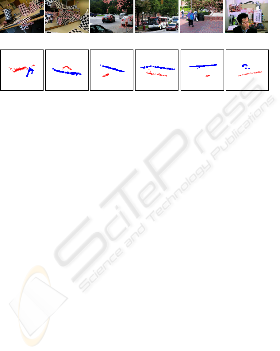
24 frames

330 points

29 frames

225 points

30 frames

502 points

31 frames

159 points

30 frames

469 points

100 frames

73 points

(a) (b) (c) (d) (e) (f)

Figure 4: Top: Feature points detected from 6 video streams of the Hopkins155 database. Bottom: Their their 3-D represen-

tation.

REFERENCES

Costeira, J. P. and Kanade, T. (1998). A multibody factor-

ization method for independently moving objects, Int.

J. Computer Vision, 29, 159–179.

Fan, Z., Zhou, J. and Wu, Y. (2006). Multibody grouping

by inference of multiple subspace from high-

dimensional data using oriented-frames, IEEE Trans

Patt. Anal. Mach. Intell., 28, 91–105.

Gear, C. W. (1998). Multibody grouping from motion im-

ages, Int. J. Comput. Vision, 29, 133–150.

Ichimura, N. (1999). Motion segmentation based on fac-

torization method and discriminant criterion, Proc. 7th

Int. Conf. Comput. Vis., Vol. 1, Kerkyra, Greece, 600–

605.

Ichimura, N. (2000). Motion segmentation using feature

selection and subspace method based on shape space,

Proc. 15th Int. Conf. Pattern Recog., Vol. 3, Barcelona,

858–864.

Inoue, K. and Urahama, K. (2001). Separation of multiple

objects in motion images by clustering, Proc. 8th Int.

Conf. Comput. Vis., Vol. 1, Vancouver, 219–224.

Kanatani, K. (2002a). Evaluation and selection of models

for motion segmentation, Proc. 7th Euro. Conf. Com-

put. Vis., Vol. 3, Copenhagen, 335–349.

Kanatani, K. (2001). Motion segmentation by subspace

separation and model selection, Proc. 8th Int. Conf.

Comput. Vis., Vol. 2, Vancouver, 301–306.

Kanatani, K. (2002b). Motion segmentation by subspace

separation: Model selection and reliability evaluation,

Int. J. Image Graphics, 2, 179–197.

Kanatani, K. (1996). Statistical Optimization for Geomet-

ric Computation: Theory and Practice, Amsterdam:

Elsevier. Reprinted (2005) New York: Dover.

Kanatani, K. (2008). Statistical optimization for geometric

ﬁtting: Theoretical accuracy analysis and high order er-

ror analysis, Int. J. Comput. Vision, 80, 167–188.

Kanatani, K. and Sugaya, Y. (2007). Performance evalua-

tion of iterative geometric ﬁtting algorithms, Comp.

Stat. Data Anal., 52, 1208–1222.

Poelman, C. J. and Kanade, T. (1997). A paraperspective

factorization method for shape and motion recovery,

IEEE Trans. Pattern Anal. Mach. Intell., 19, 206–218.

Rao, S. R., Tron, R., Vidal R. and Ma, Y. (2008). Motion

segmentation via robust subspace separation in the

presence of outlying, incomplete, or corrupted trajec-

tories, Proc. IEEE Conf. Comput. Vision Patt. Recog.,

Anchorage, AK.

Schindler, K., Suter, D. and Wang, H. A model-selection

framework for multibody structure-and-motion of

image sequences, Int. J. Comput. Vision, 79, 159–177.

Sugaya, Y. and Kanatani, Y. (2004). Multi-stage optimiza-

tion for multi-body motion segmentation. IEICE Trans.

Inf. & Syst., E87-D, 1935–1942.

Taubin, G. (1991). Estimation of planer curves, surfaces,

and non-planar space curves deﬁned by implicit equa-

tions with applications to edge and range image seg-

mentation, IEEE Trans. Patt. Anal. Mach. Intell., 13,

1115–1138.

Tomasi, C. and Kanade, T. (1992). Shape and motion from

image streams under orthography—A factorization

method, Int. J. Comput. Vision, 9, 137–154.

Tron, R. and Vidal, R. (2007). A benchmark for the com-

parison of 3-D motion segmentation algorithms, Proc.

IEEE Conf. Comput. Vision Patt. Recog., Minneapolis,

MN.

Vidal, R., Ma, Y. and Sastry, S. (2005). Generalized prin-

cipal component analysis (GPCA), IEEE Trans. Patt.

Anal. Mach. Intell., 27, 1945–1959.

Vidal, R. Tron, R. and Hartley, R. (2008). Multiframe mo-

tion segmentation with missing data using PowerFac-

torization and GPCA, Int. J. Comput. Vision, 79, 85–

105.

Wu, Y. Zhang, Z., Huang, T. S. and Lin, J. Y. (2001).

Multibody grouping via orthogonal subspace decom-

position, sequences under afﬁne projection, Proc.

IEEE Conf. Computer Vision Pattern Recog., Vol. 2,

Kauai, HI, 695–701.

Yan, J. and Pollefeys, M. (2006). A general framework for

motion segmentation: Independent, articulate, rigid,

non-rigid, degenerate and nondegenerate, Proc. 9th

Euro. Conf. Comput. Vision., Vol. 4, Graz, Austria,

94–104.

VISAPP 2010 - International Conference on Computer Vision Theory and Applications

206