MODELING RADIAL VELOCITY SIGNALS FOR EXOPLANET

SEARCH APPLICATIONS

Prabhu Babu

∗

, Petre Stoica

Division of Systems and Control, Department of Information Technology

Uppsala University, P.O. Box 337, SE-75 105, Uppsala, Sweden

Jian Li

Department of Electrical and Computer Engineering, University of Florida, Gainesville, 32611, FL, U.S.A.

Keywords:

Radial velocity method, Exoplanet search, Kepler model, IAA, Periodogram, RELAX, GLRT.

Abstract:

In this paper, we introduce an estimation technique for analyzing radial velocity data commonly encountered in

extrasolar planet detection. We discuss the Keplerian model for radial velocity data measurements and estimate

the 3D spectrum (power vs. eccentricity, orbital period and periastron passage time) of the radial velocity data

by using a relaxation maximum likelihood algorithm (RELAX). We then establish the signiﬁcance of the

spectral peaks by using a generalized likelihood ratio test (GLRT). Numerical experiments are carried out on

a real life data set to evaluate the performance of our method.

1 INTRODUCTION

Extrasolar planet (or shortly exoplanet) detection is

a fascinating and challenging area of research in the

ﬁeld of astrophysics. Till mid 2009, 353 exoplanets

have been discovered. Some of the techniques avail-

able in the astrophysics literature to detect exoplanets

are astrometry, the radial velocity method, pulsar tim-

ing, the transit method and gravitational microlens-

ing. Among these methods, the radial velocity analy-

sis is the most commonly used technique, in which the

Doppler shift in the spectral lines and hence the radial

velocity of the parent star is measured. The spectrum

of the measured Doppler shifts is then analyzed to de-

tect the exoplanet(s) revolving around the star.

Most often the radial velocity measurements are ob-

tained at nonuniformly spaced time intervals due to

hardware and practical constraints, which limits the

application of commonly used spectral analysis meth-

ods. The most straightforward way to deal with this

problem is to use the standard periodogram by ignor-

ing the nonuniformity of data samples, which results

in an inaccurate spectrum. In (Roberts et al., 1987), a

method named CLEAN was proposed, which is based

∗

Corresponding author. This work was supported in part

by the Swedish Research Council (VR).

on iterative deconvolution in the frequency domain to

obtain a clean spectrum from an initial dirty one. A

periodogram related method is the least squares peri-

odogram (also called the Lomb-Scargle periodogram)

(Lomb, 1976; Scargle, 1982) which estimates the si-

nusoidal components by ﬁtting them to the observed

data. Most recently, (Yardibi et al., 2010; Stoica et al.,

2009) introduced a new method called the Iterative

Adaptive Approach (IAA), which relies on solving an

iterative weighted least squares problem.

In this paper, we analyze the radial velocity data

by using a relaxation maximum likelihood algorithm

(RELAX) initialized with IAA estimates. The signif-

icance of the spectral peaks is then established via a

generalized likelihood ratio test (GLRT). Numerical

experiments are carried out on a real life radial veloc-

ity data set.

In Section 2, we describe the model used in this pa-

per for the radial velocity data. Section 3 presents the

RELAX and GLRT methods, and Section 4 contains

the results for a real life example. Finally, the paper

is concluded in Section 5.

155

Babu P., Stoica P. and Li J. (2010).

MODELING RADIAL VELOCITY SIGNALS FOR EXOPLANET SEARCH APPLICATIONS.

In Proceedings of the 7th International Conference on Informatics in Control, Automation and Robotics, pages 155-159

DOI: 10.5220/0002770601550159

 SciTePress

2 DATA MODEL

Let {y(t

)}

n=1

denote the radial velocity of a star

measured at a set of possibly nonuniform time in-

stants {t

}

n=1

. Based on the Keplerian model of plan-

etary motion (Zechmeister and Kurster, 2009) (Cum-

ming, 2004), the radial velocity data are modeled as

follows:

y(t

) = C

∑

m=1

[cos(ω

+ ν

)) + e

cos(ω

)],

n = 1, ··· , N

(1)

where C

is the constant radial velocity, and

tan(ν

)) =

1+e

1−e

tan(E

))

) − e

sin(E

)) =

2π(t

−T

)

(2)

M: Number of exoplanets revolving around the

star. The number of planets M is usually unknown.

: Eccentricity of the orbit of the m

planet.

: Longitude of the periastron for the m

planet.

: Orbital period of the m

planet; P

is related

to orbital frequency f

by f

: Periastron passage time of the m

planet.

: Radial velocity amplitude of the m

planet.

), E

): True and eccentric anomaly of the

planet, with t

denoting their time dependence.

We divide the entire 2D space G , deﬁned as G =

{(e, f), 0 ≤ e < e

max

, −

max

< f <

max

}, into a grid

of prespeciﬁed size K. We point out here that the grid

G does not include the parameter T, and that T is

taken to be zero for the time being but will be esti-

mated as described later on. The choices of e

max

and

max

in G depend on the sampling pattern: to deter-

mine them, we calculate the spectral window deﬁned

as:

W(e, f) =



∑

n=1

exp( jν(t

))



, 0 ≤ e < 1, −∞ ≤ f ≤ ∞.

(3)

For any choice of (e, f) and t

, there exists a ν(t

) ob-

tained via (2). Following (Eyer and Bartholdi, 1999),

the parameters e

max

and f

max

are chosen such that the

region G leads to an unambiguousW(e, f) (see (Babu

et al., 2010) for more details).

3 PARAMETER ESTIMATION

AND STATISTICAL

SIGNIFICANCE TESTING:

RELAX AND GLRT

The estimates obtained from IAA are usually fairly

accurate. However, if the grid (G ) is not chosen ﬁne

enough (to reduce the computation time), then IAA

might miss some true peaks (see (Babu et al., 2010)

for an elaborate discussion on IAA for radial veloc-

ity data). In that case, applying RELAX (Li and

Stoica, 1996), a parametric iterative estimation al-

gorithm, can reﬁne the IAA estimates. Algorithm 1

brieﬂy describes the steps involved in RELAX. The

P largest peaks picked from IAA are used as initial

estimates for RELAX, which has a beneﬁcial effect

on the convergence of RELAX compared with using

other more arbitrary initial estimates. In the case of

radial velocity data, the choice of P = 5 peaks ap-

pears to be reasonable for most applications. RELAX

generally converges within a few iterations (typically

in less than 10 iterations).

Next we note that, under the assumption the noise

in the data is Gaussian distributed, the RELAX esti-

mates are optimal in the maximum likelihood sense

(Li and Stoica, 1996). We can then use the general-

ized likelihood ratio test (GLRT) to establish the sta-

tistical signiﬁcance of the estimated planet parame-

ters. We ﬁrst apply RELAX to the largest IAA peak

and use GLRT to test the null hypothesis that there are

no planets (or, in other words, that the data is made

only of white noise) against the hypothesis that there

is at least one exoplanet. If the test rejects the null

hypothesis then we will proceed and apply RELAX

to the two largest peaks and subsequently test the hy-

pothesis that there is one exoplanet in the data against

the hypothesis that there are at least two exoplanets;

and so on. As an example, for the following hypothe-

ses

: There are no planets.

: There is at least one exoplanet with eccentricity

ˆe

, orbital frequency

and periastron passage time

the log-likelihood (LL) functions are given by:

LL(H

) =

−



∑

n=1

|y(t



+C,

LL(H

) =

−



∑

n=1

|y(t

) − ˆr

cos(ν(t

)) − ˆq

sin(ν(t

))|



(4)

where C is an additive constant, ν(t

) is calculated

from the RELAX estimates (ˆe

), and ˆr

, ˆq

are the least square estimates of r, q corresponding to

(ˆe

), see Algorithm 1. Under the assumption

that hypothesis H

is true, the log-likelihood-ratio,

deﬁned as 2(LL(H

) − LL(H

)), is asymptotically a

random variable with a chi-square distribution. Then

the GLRT is given by

2(LL(H

) − LL(H

))

≷

(5)

ICINCO 2010 - 7th International Conference on Informatics in Control, Automation and Robotics

156

where Λ denotes a ﬁxed threshold. The threshold is

usually chosen such that prob(X ≤ Λ) = ξ, where X ∼

denotes a chi-square distributed random variable

with 5 degrees of freedom (because of the 5 unknowns

per planet in the data model, namely e, f, T, r and

q), and ξ determines the signiﬁcance level of the test.

Choosing ξ = 0.99 gives a false alarm probability of

0.01 and the corresponding threshold is Λ = 15.

4 A REAL LIFE EXAMPLE:

HD 208487

In this section, we consider the application of the al-

gorithm introduced in the previous section to a real

life radial velocity data set. Our goal is to detect

the exoplanets present in a star system and estimate

their eccentricities, frequencies and periastron pas-

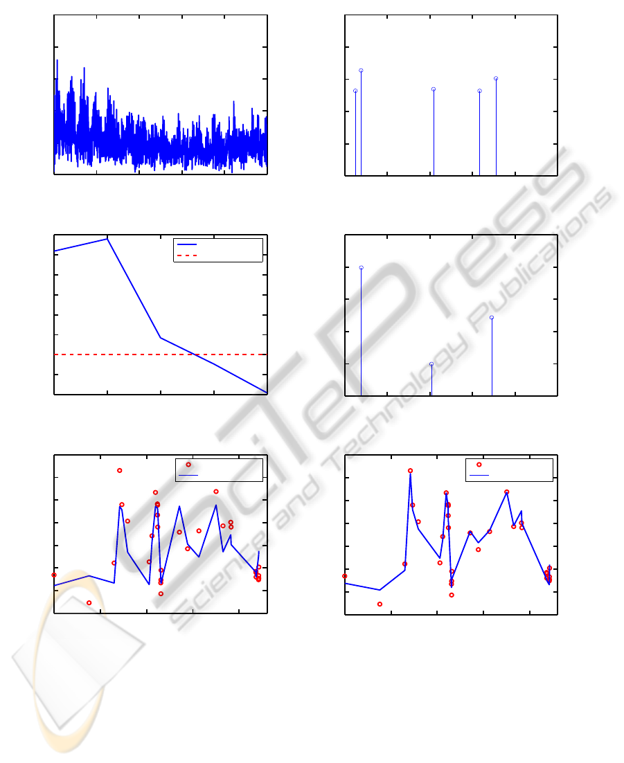
sage times. We will show the following plots:

• Amplitude vs. orbital frequency for IAA and

RELAX (eccentricity and periastron passage time

values for the peaks in the amplitude spectrum are

indicated in the plots).

• Likelihood ratio vs. the planet number.

• Observed and ﬁtted data sequences.

The data set used here consists of 31 samples of

radial velocity measurements of the star HD 208487.

The parameters e

max

and f

max

are determined from

the spectral window to be 0.5 and 1 cycles/day. The

spectrum obtained using IAA is shown in Fig.1(a),

which indicates the presence of more than one planet.

The 5 largest peaks in the IAA spectrum are picked

up and are used to initialize RELAX. The GLRT

plot shown in Fig.1(c) suggests the existence of three

planets in the HD 208487 star system with the fol-

lowing parameters (see Fig.1(d) and also Table 1):

= 0.326, f

= 0.0078 cycles/day, T

= 130.9

days), (e

= 0.315, f

= 0.069 cycles/day, T

= 14.2

days) and (e

= 0, f

= 0.0408 cycles/day, T

= 2.9

days). However (Tinney et al., 2005) reported that the

star has only one planet with an orbital frequency of

0.0077 cycles/day. Fig. 1(e) and 1(f) showthe plots of

measured data and the ﬁtted data obtained assuming

the existence of one and, respectively, three planets. It

is seen clearly from these ﬁgures that the three planet

model ﬁts the measured data much better than a single

planet model.

5 CONCLUSIONS

The real life example discussed in the paper suggests

that our algorithm successfully detects the presence

of spectral peaks (planets) in radial velocity data and

accurately identiﬁes both their frequencies and eccen-

tricities as well as their periastron passage times. The

example used here is typical of cases usually encoun-

tered in exoplanet search and hence the proposed al-

gorithm is believed to be an effective and useful tool.

REFERENCES

Babu, P., Stoica, P., Li, J., Chen, Z., and Ge, J. (2010).

Analysis of radial velocity data by a novel adaptive

approach. The Astronomical Journal, 139:783–793.

Cumming, A. (2004). Detectability of extrasolar planets in

radial velocity surveys. Monthly Notices of the Royal

Astronomical Society, 354(4):1165–1176.

Eyer, L. and Bartholdi, P. (1999). Variable stars: Which

Nyquist frequency? Astronomy and Astrophysics,

Supplement Series, 135:1–3.

Li, J. and Stoica, P. (1996). Efﬁcient mixed-spectrum es-

timation with applications to target feature extraction.

IEEE Transactions on Signal Processing, 44(2):281–

295.

Lomb, N. R. (1976). Least-squares frequency analysis of

unequally spaced data. Astrophysics and Space Sci-

ence, 39(1):10–33.

Roberts, D. H., Lehar, J., and Dreher, J. W. (1987). Time

series analysis with CLEAN. I. Derivation of a spec-

trum. The Astronomical Journal, 93(4):968–989.

Scargle, J. D. (1982). Studies in astronomical time se-

ries analysis. II. Statistical aspects of spectral analy-

sis of unevenly spaced data. Astrophysical Journal,

263:835–853.

Stoica, P., Li, J., and He, H. (2009). Spectral analysis of

nonuniformly sampled data: A new approach versus

the periodogram. IEEE Transactions on Signal Pro-

cessing, 57(3):843–858.

Stoica, P. and Moses, R. (2005). Spectral Analysis of Sig-

nals. Prentice Hall, Upper Saddle River, N.J.

Tinney, C., Butler, R., Marcy, G., Jones, H., Penny, A., Mc-

Carthy, C., Carter, B., and Fischer, D. (2005). Three

Low-Mass Planets from the Anglo-Australian Planet

Search 1. The Astrophysical Journal, 623(2):1171–

1179.

Yardibi, T., Li, J., Stoica, P., Xue, M., and Baggeroer, A. B.

(2010). Iterative adaptive approach for sparse sig-

nal representation with sensing applications. IEEE

Transactions on Aerospace and Electronic Systems,

46:425–443.

Zechmeister, M. and Kurster, M. (2009). The generalised

Lomb-Scargle periodogram. Astronomy and Astro-

physics, 496(2):577–584.

MODELING RADIAL VELOCITY SIGNALS FOR EXOPLANET SEARCH APPLICATIONS

157

APENDIX

0 0.1 0.2 0.3 0.4 0.5

Orbital frequency (cycles/day)

Amplitude

0 0.02 0.04 0.06 0.08 0.1

Orbital frequency (cycles/day)

Amplitude

(0, 83.4)

(0, 102)

(0, 2.1)

(0.44, 15.4)

(0.2, 13.8)

(a) (b)

1 2 3 4 5

Number of peaks

Likelihood ratio

Threshold

0 0.02 0.04 0.06 0.08 0.1

Orbital frequency (cycles/day)

Amplitude

(0.326, 130.9)

(0, 2.9)

(0.315, 14.2)

0 500 1000 1500 2000

−30

−20

−10

Time (days)

Amplitude

Observed data

Fitted data

0 500 1000 1500 2000

−30

−20

−10

Time (days)

Amplitude

Observed data

Fitted data

(e) (f)

Figure 1: HD 208487: (a) the IAA spectrum, (b) the 5 largest peaks in the IAA spectrum, (c) the likelihood ratio, (d) the

RELAX spectrum, (e) comparison of the observed data and ﬁtted data obtained from the parameters of the planet reported in

(Tinney et al., 2005) and (f) comparison of the observed data and ﬁtted data obtained from the three detected planets.

ICINCO 2010 - 7th International Conference on Informatics in Control, Automation and Robotics

158

Table 1: Parameters of the planets of HD 208487 star system.

∗)

The third planet becomes statistically insigniﬁcant if the false

alarm probability is decreased from 10

−2

to 10

−4

, in which case the threshold becomes Λ = 25.

Planet No. Previous work This work

e f(cycles/day) T(days) β e f(cycles/day) T(days) β

1 0.24 0.0077 92 20 0.3260 0.0078 130.9 19.9

2 - - - - 0.3150 0.0690 14.2 12.18

∗)

- - - - 0 0.0408 2.9 4.96

Algorithm 1: RELAX.

Let {(e

, f

, T

)}

p=1

denote the parameters of the P most dominant planets in the IAA spectrum (e.g. P = 5).

The initial values of their radial velocity amplitudes {(r

, q

)}

p=1

are taken to be zero.

for p = 1 to P do

for i = 1 to I (e.g. I = 10) do

for u = 1 to p do

) = y(t

)−

∑

k=1,k6=u



i−1

cos(ν

i−1

)) + q

i−1

sin(ν

i−1

))



where ν

i−1

is obtained from

i−1

, f

i−1

, T

i−1

). Then

, f

, T

)

= argmin

{e, f ,T}

min

{r,q}

∑

n=1



) −r cos(ν(t

)) − qsin(ν(t

))



The inner minimization with respect to {r, q} in the above equation is a least squares problem and the

estimates {r

, q

} can be obtained analytically (see (Stoica and Moses, 2005)). The minimization with

respect to {e, f, T} is carried out via a 3D grid search performed around (e

i−1

, f

i−1

, T

i−1

end for

for u = 1 to p do

, f

, T

) ← (e

, f

, T

) and (r

, q

) ← (r

, q

end for

{( ˆe

) ← (e

, f

, T

)}

p=1

and {(ˆr

, ˆq

) ← (r

, q

)}

p=1

MODELING RADIAL VELOCITY SIGNALS FOR EXOPLANET SEARCH APPLICATIONS

159