
MODELING COMPLEXITY OF PHYSIOLOGICAL TIME SERIES
IN-SILICO
Jesse Berwald, Tom
´
a
ˇ
s Gedeon
Department of Mathematics, Montana State University, Bozeman, Montana, U.S.A.
Konstantin Mischaikow
Department of Mathematics and BioMaPS Institute, Rutgers University, Piscataway, New Jersey, U.S.A.
Keywords:
Physiological time series, Complexity, Neural networks.
Abstract:
A free-running physiological system produces time series with complexity which has been correlated to the
robustness and health of the system. The essential tool to study the link between the structure of the system and
the complexity of the series it produces is a mathematical model that is capable of reproducing the statistical
signatures of a physiological time series. We construct a model based on the neural structure of the hippocam-
pus that reproduces detrended fluctuations and multiscale entropy complexity signatures of physiological time
series. We study the dependence of these signatures on the length of the series and on the initial data.
1 INTRODUCTION
Measuring an output of a physiological system pro-
vides a window into its complex multi-scale dynam-
ics. The measurements are often spread over time and
many techniques of time series analysis have been
used to gain an insight into the underlying physiol-
ogy. Some of the most intriguing observations indi-
cate that the complexity of the time series produced
by a free-running physiological system, as measured
by Detrended Fluctuation Analysis (DFA), Multiscale
Entropy (MSE) and other methods, is correlated to
the robustness and health of the physiological system.
More precisely, analysis of time series gathered from
the measurement of cardiac inter-beat intervals, oscil-
lations of red blood cells, gait analysis, and other pat-
terns observed in living organisms (Goldberger, 2006;
Goldberger et al., 2000; Costa et al., 2002; Costa
et al., 2005; Peng et al., 1994; Peng et al., 2007) sug-
gests that healthy systems produce complex time se-
ries, while compromised systems produce either very
simple periodic signals, or completely random sig-
nals.
The potential diagnostic and therapeutic conse-
quences of this hypothesis demand studies that go be-
yond passive analysis of existing data. What is needed
is a model which reproduces observed characteristics
of physiological signals and thence can be actively
tested. Ideally, such a model would be based on our
knowledge of a complex system. However, it has
proved challenging to construct a dynamical system-
based model that reproduces the statistical character-
istics of physiological time series. The only success-
ful attempt was a discrete map with added noise (Peng
et al., 2007) which partially reproduced some of these
characteristics.
The central aim of our work is to construct a de-
terministic FitzHugh-Nagumo-based neural network
model which exhibits the complex signatures mea-
sured by DFA and MSE metrics in physiological sig-
nals. We study the dependence of these metrics on the
length of the computed time series and initial condi-
tions used. Note that this issue has relevance to the
analysis of experimental time series. One tacitly as-
sumes that the analyzed series represents the steady
response of the system, which does not depend on ini-
tial data, or the time when the measurements started.
The longer the time series, the more time the sys-
tem has for the initial data effect to “average out”.
While these assumptions are satisfied if the determin-
istic system is ergodic and stationary, we can test them
directly in our model.
The model consists of a network of five excitatory
cells and five inhibitory cells. The structure and dy-
namics of the network are based on the work of Ter-
man (Terman et al., 2008) modeling the structure of
61
Berwald J., Gedeon T. and Mischaikow K. (2010).
MODELING COMPLEXITY OF PHYSIOLOGICAL TIME SERIES IN-SILICO.
In Proceedings of the Third International Conference on Bio-inspired Systems and Signal Processing, pages 61-67
DOI: 10.5220/0002710300610067
Copyright
c
SciTePress

the hippocampus. Analyzing the time series of av-
erages from the excitatory cells’ voltage potential, we
show that it matches the DFA and MSE measurements
of complexity for free-running physiological systems
across a range of time scales. These results do not de-
pend on the initial conditions used. Furthermore, we
show that the range of complex behavior grows when
we increase the length of the time series from 15,000
to 100,000 (in arbitrary units), but does not grow fur-
ther, when we extend the length to 400,000.
This indicates that the system has a certain capac-
ity for complexity which does not depend on initial
conditions, and which is recovered from data of finite
length.
2 NEURAL NETWORK MODEL
We create a bipartite graph G = hV
E
,V
I
,Ai, where V
E
consists of excitatory nodes, or cells, V
I
consists of in-
hibitory cells, and A is the set of directed edges which
consists of the following types of connections:
e
j
→ i
k
, i
k
→ e
j
, and i
k
→ i
k
0
, k 6= k
0
,
where e denotes an excitatory cell and i denotes an in-
hibitory cell; j ∈ {1, .. .,n} and k,k
0
∈ {1, ...,m},and
n = |V
E
|, m = |V
I
|. Excitatory cells do not connect to
other excitatory cells in order to avoid the blow-up of
the solutions due to runaway positive feedback. The
subgraph V
I
is complete. We construct the remaining
connections randomly by selecting the e
j
→ i
k
and
i
k
→ e
j
edges with probability ρ = (lnN)/N, where
N = n + m. Figure 1 shows a sample neural net-
work. Edges are weighted by a maximal conductance
constant which depends on the type of connection.
We represent these weights by g
IE
, g
EI
, g
II
∈ (0,1),
where the subscripts E and I denote excitatory and
inhibitory edges, respectively, and g
xy
specifies the
weight for the directed edge x → y.
2.1 FitzHugh-Nagumo Equations
The following system of coupled differential equa-
tions describes the behavior of each cell in the graph
defined above (Terman et al., 2008). All units are ar-
bitrary.
Inhibitory cells:
dv
dt
= v −
v
3
3
− w − g
II
(v − v
I
)
∑
s
k
− g
EI
(v − v
E
)
∑
s
j
+ K
I
(t)
dw
dt
= ε(v − bw + c)
5 3
2
4
2
1
1
5
4
3
Figure 1: A neural network with ten cells. Inhibitory cells
(I) are represented by blue squares, excitatory cells (E) by
red ellipses. The subgraph of I cells is completely con-
nected. E → I and I → E edges are created with probability
lnN
N
. E → E edges are not allowed.
ds
dt
= α
I
(1 − s)h(x,θ
x
) − β
I
s
dx
dt
= ε[α
x
(1 − x)h(v,θ
I
) − β
x
x]. (1)
Excitatory cells:
dv
dt
= v −
v
3
3
− w − g
IE
(v − v
I
)
∑
s
k
+ K
E
(t)
dw
dt
= ε(v − bw + c)
ds
dt
= α(1 − s)h(v,θ) − βs, (2)
In general, the coupling variable s represents the frac-
tion of open synaptic channels. The coupling sums,
∑
s
k
and
∑
s
j
, are limited to those cells connecting to
the given cell; s
k
is the input from an inhibitory cell,
s
j
is the input from an excitatory cell.
A direct synapse is one in which the postsynap-
tic receivers are themselves ion channels. In equa-
tions (2) an excitatory cell is modeled with a direct
synapse. The function h is a steep sigmoidal curve al-
lowing for a very rapid, but still continuous, activation
of the synaptic processes. Once the voltage potential
v crosses θ the synapse activates (h turns on) and an
impulse travels to connected cells.
An indirect synapse, where the postsynaptic re-
ceivers are not ion channels, is modeled by adding the
delay variable x. All inhibitory synapses in our model
are indirect. The activation of the synaptic variable s
relies on x, not v as in a direct synapse. In the bot-
tom equation of (1), v must first reach the threshold
θ
I
in order to activate x. After this delay, x goes on to
activate s.
Each cell is assigned a unique ε 1. If the cell
oscillates when disconnected from the other cells, ε
BIOSIGNALS 2010 - International Conference on Bio-inspired Systems and Signal Processing
62
0
5000
10000
15000
Time (arbitrary units)
-2
-1.5
-1
-0.5
0
0.5
Average voltage potential
(a)
0.5
1
1.5
2
2.5
3
log(w)
-1
0
1
log F(w)
log F(w)
Linear reg slope = 1.41
Linear reg slope = 1.063
(b)
0 10 20 30
τ
0.2
0.25
0.3
0.35
0.4
0.45
SE(τ)
(c)
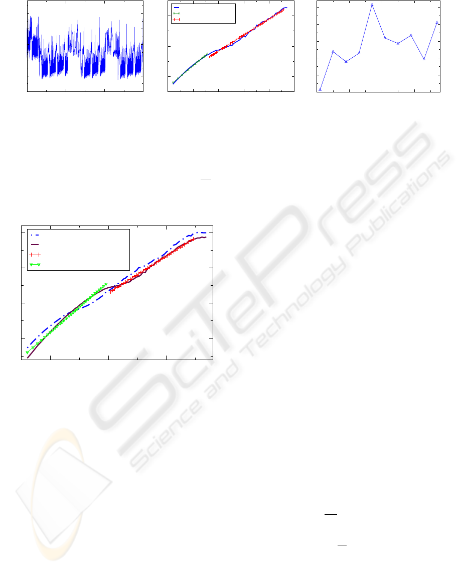
Figure 2: (a) Time series for a simulation run for 15000 “seconds” (units are arbitrary). (b) The DFA curve exhibits two trends:
at short scales we observe autocorrelation effects due to deterministic ODE solver, at longer scales we find a scaling exponent
of β = 1.063, similar to physiological systems, though over a shorter range. The relatively short time series produces more
variability in the higher window sizes since the number of data points used to calculate the DFA becomes small. (c) Sample
entropy SE(τ) = SE(m, δ, N, τ) is calculated for τ = 1,5,.. . , 37, m = 7, and δ = 0.2. The length, N, of the coarse-grained time
series depends on τ. The MSE curve has an average of SE = 0.35. The variance of Var(SE) = 0.003 is larger than in longer
simulations. As in (b), this greater variability is due to the relatively small number of data points in the original time series.
1 2 3
log(w)
-1
0
1
2
log F(w)
log F(w)
log F(w), ε/10
Linear reg slope = 1.05
Linear reg slope = 1.43
Figure 3: DFA curve from an initial ε distribution (solid
blue), and the DFA curve obtained by dividing each ε by 10
(dashed purple).
is inversely proportional to the period of this oscilla-
tion. The constants v
E
and v
I
are reversal potentials
for excitatory and inhibitory cells, respectively. The
maximal conductance constants g
IE
, g
EI
, g
II
weight
a cell’s input by multiplying the coupling terms.
The parameters α,α
I
, α
x
, β, β
I
, β
x
∈ R are rates
at which the synaptic variables, s and x, turn on and
off. The linear recovery term is specified by the pa-
rameters b, c ∈ R. And the K
E
and K
I
terms represent
external input to the system. In order for cells to enter
an excitatory state a small amount of input must be
applied to the system. For simplicity we use constant
input. The complete set of parameters used is listed
in the Appendix.
2.2 In-Silico Neural Network
An in-silico neural network, N is constructed from
the following constituent pieces. The structure and
behavior of the network is specified in a graph G com-
posed of cells whose behavior is described by (1) and
(2). A parameter set P contains fixed parameters for
the FitzHugh-Nagumo equations. Thus, hG,Pi gener-
ate a unique neural network N used for simulations.
3 TIME SERIES ANALYSIS
Solving the above system of ODE’s with an adaptive
step solver results in a set of solutions for each cell.
The voltage potentials, v
j
(t), from all excitatory cells
are averaged at each time step to give a time series
g(t). The analysis techniques require equally spaced
time steps. Since an adaptive step algorithm returns
irregularly spaced time steps we construct a new time
series by partitioning the time axis into bins and aver-
aging over these bins, giving a time series composed
of the values
¯g(n) =
1
κT
(n+1)(κT )
∑
i=n(κT )
g(i), (3)
where n = 0, 1,.. .,L = b
M
κT
c, M is the length of g(t),
and κ is chosen so that each bin contains a minimum
number of points. Note that a small tail of the original
time series must be discarded. We apply the following
techniques to series ¯g(n).
MODELING COMPLEXITY OF PHYSIOLOGICAL TIME SERIES IN-SILICO
63

0 20000 40000
60000
80000
1e+05
Time (arbitrary units)
-2
-1.5
-1
-0.5
0
0.5
Average voltage potential
(a)
1 2 3
log(w)
-1
0
1
2
log F(w)
log F(w)
Linear reg slope = 1.382
Linear reg slope = 1.097
Linear reg slope = 0.12
(b)
0 10 20 30
τ
0.2
0.25
0.3
0.35
0.4
SE(τ)
(c)
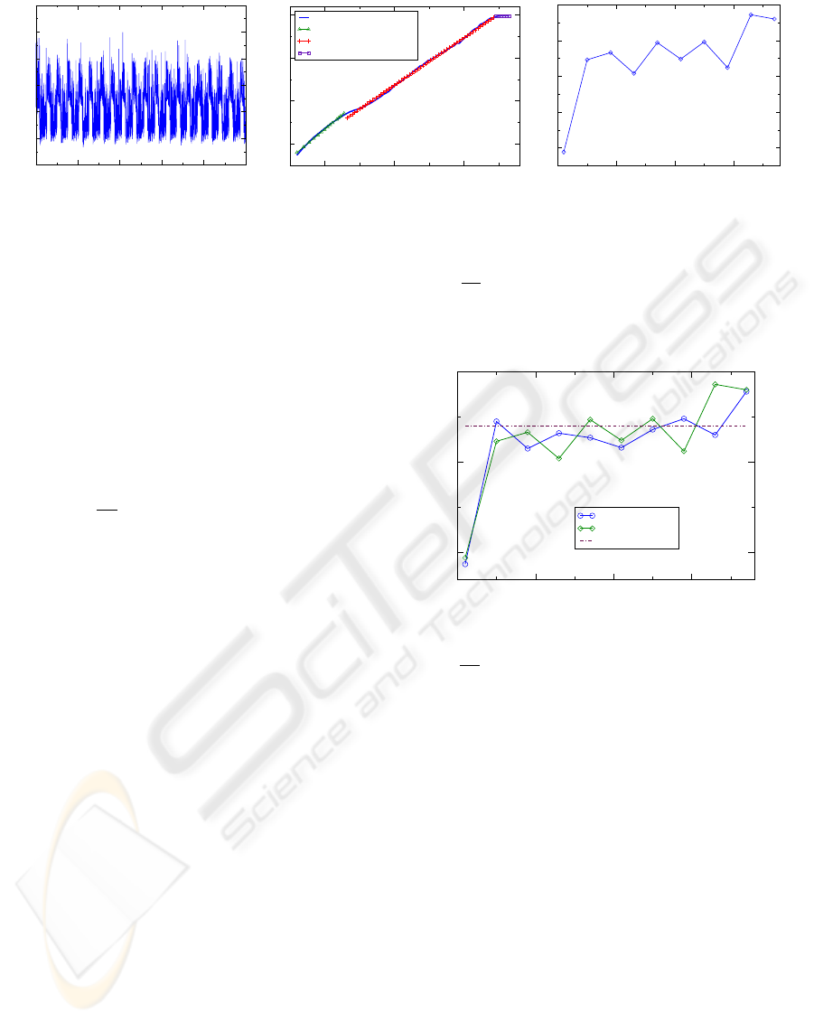
Figure 4: (a) Time series from simulating N for 100000. (b) The region of physiological complexity for the DFA curve
extends from w = 10
1.3
to w = 10
3.5
. For windows larger than 10
3.5
we observe a new, flat trend indicating that the time
series generated by N is devoid of long range correlations for these larger windows. (c) The MSE curve is relatively constant
over a large number of scales indicating physiological complexity in the time series. The average sample entropy for τ ≥ 5 is
SE = 0.34, with a variance of Var(SE) = 0.0007.
3.1 Detrended Fluctuation Analysis
Detrended fluctuation analysis is a statistical method
developed to determine long term trends in time series
(Peng et al., 1994; Peng et al., 1995). Given a time
series of length N, it is first integrated at each point to
give a function y(t) =
R
t
0
g(s)ds. The time axis is then
partitioned into windows of length w. Next, a linear
regression line, y
w
(t), is fit to the integrated curve for
each window. The root-mean-square of the detrended
curve y(t) − y
w
(t) is calculated, giving the detrended
fluctuation value for a window size w:
F(w) =
s
1
N
N
∑
k=0
(y(t) − y
w
(t))
2
,
where y
w
is understood to be the linear regression to
y defined piecewise over each window of length w.
F is computed for a wide range of window sizes and
typically increases monotonically. Power law scaling
exists in the time series when a log-log plot produces
a linear relationship.
3.2 Multiscale Entropy
Multiscale entropy (Costa et al., 2005; Costa et al.,
2002) simulates the sequence of refinements in the
definition of Kolmogorov-Sinai (KS) entropy (Katok
and Hasselblatt, 1997). In the case of MSE, though,
we are interested in the evolution of the entropy across
these refinements, and not their limit. Suppose we
obtain a time series g(t) by taking measurements of
an experiment. This gives a sequence of data points
{g(0),g(1),... ,g(N)}. MSE simulates the situation
where we perform the identical experiment with less
time accuracy. A time series for this situation is con-
structed through coarse graining, or partitioning the
time axis of the original series into blocks of size
τ ∈ N and averaging the data over these windows.
Thus, each coarse grained time series is composed of
the points
g
τ
(n) =
1
τ
(n+1)τ
∑
k=nτ
g(k),
where n = 0,1,... ,L = bN/τc.
The entropy of this new time series
{g
τ
(0),g
τ
(1),..., g
τ
(L)} is estimated using sam-
ple entropy (Richman and Moorman, 2000). Sample
entropy views a time series as a sequence of random
variables and measures the creation of information
by computing the correlation between delay vectors
of length m and m + 1.
In order to define sample entropy, fix τ and set
g
τ
(i) = x
i
. Given m, let u
m
(i) = {x
i
,x
i+1
,. .., x
i+m
}
be a delay vector of length m, and define the num-
ber of vectors close to u
m
(i) as n
m
i
(δ) = #{x
m
( j) :
d(x
m
(i),x
m
( j)) < δ} where δ > 0 is some tolerance
and d = max
k=0,1,...,m
{| x
m
(i+k)−x
m
( j +k) |}. There
are N(m) = L − m full length vectors u
m
( j), exclud-
ing the possibility of self matches. The probability of
finding the vector u
m
( j) within a distance δ of u
m
(i)
is
C
m
i
(δ) =
n
m
i
(δ)
N(m)
.
For the parameter m the probability that any two vec-
tors are within δ of each other is
C
m
(δ) =
1
N(m)
N(m)
∑
i=0
C
m
i
(δ)
The above correlation integral is used to define the
sample entropy for the delay m, tolerance δ, and time
series length L as
SE(m, δ,L) = −ln
C
m+1
C
m
.
BIOSIGNALS 2010 - International Conference on Bio-inspired Systems and Signal Processing
64

C
m+1
/C
m
is commonly thought of as the informa-
tion gained as the trajectory moves from time mτ to
(m + 1)τ. A larger difference between C
m
and C
m+1
results in more information, i.e., a higher value of SE.
For a fixed value of m the graph of the sample entropy
over a range of τ’s provides a measure of the amount
of long range correlation in the time series. A rela-
tively constant amount of entropy across many values
of τ signifies correlations amongst data points over
multiple time scales. For instance, 1/ f noise which is
highly correlated across time scales yields a constant
MSE curve. In contrast, white noise is monotonically
decreasing since it possesses no long range correla-
tions.
4 RESULTS
Consider an in-silico neural network N as defined in
Section 2.2. We construct the time series of voltage
potentials ¯g(n) by choosing a set of initial conditions
and solving the system of differential equations over
the time interval [0, N], then performing the binning
procedure described in (3). The units of time are ar-
bitrary.
Figure 2 shows the time series, DFA curve, and
MSE curve for a simulation of N run for N = 15000.
In Figure 2(b), the scaling exponent β = 1.063 over
the range of window sizes w = 10
1.3
to w = 10
2.7
.
Thus, running N for a relatively short simulation pro-
duces power law scaling similar to a physiological
system over the range (1.3,2.7) for the total length of
range 1.4 . This range of scales where β ≈ 1 is shorter
than that typically seen in biological systems, where
the range typically has length greater than 3. The DFA
curve extracted from our simulations has three dis-
tinct regions. In the first region, where w < 10
1.3
, the
linear regression deviates from the power law β ≈ 1
due to autocorrelation effects on short scales, which
are caused by the deterministic ODE solver. These
effects dominate at scales much smaller than the high-
est frequency cellular oscillations, which can be esti-
mated from the largest ε. Figure 3 illustrates this ef-
fect; we compare the DFA curve in Figure 4(b) to the
curve obtained after dividing by 10 all of the ε’s used
in generating Figure 4(b). The deterministic portion
extends to higher scales because the highest oscilla-
tion frequency decreased by a factor of ten. This also
illustrates the importance of the choice of ε’s on the
DFA curve. In order to avoid these deterministic ef-
fects we focus (for the original set of ε’s listed in the
Appendix) on power law scaling in the second region,
where w > 10
1.3
.
In Figure 2(b) we see that N produces physiologi-
1 2 3 4
log(w)
-1
0
1
2
log F(w)
log F(w)
Linear reg slope = 1.37
Linear reg slope = 1.091
Linear reg slope = 0.031
Figure 5: The DFA curve after simulating N for N =
400000. The region of complexity remains unchanged from
that seen in Figure 4(b). This implies that N has an inherent
limit for generating long range correlations.
cally complex behavior in the region w > 10
1.3
, which
ends at w = 10
2.7
. By increasing the length of the
time series (Figure 4(b)) the second region extends
past w = 10
2.7
to w = 10
3.5
showing that N continues
to introduce complexity into the time series past the
scale limits imposed by the short simulation in Fig-
ure 2. The second region terminates in Figure 4(b)
at w = 10
3.5
, where a third region with no long range
correlation begins. Extending the length of the sim-
ulation to N = 400000 yields the DFA curve in Fig-
ure 5, where this third region extends to larger win-
dow sizes. Clearly the extension of the time series
fails to find longer range correlations in the time se-
ries. We conclude that the system N has an upper
limit w = 10
3.5
on the length of long range correla-
tions it can generate.
The longer time series yields an MSE curve that is
relatively constant, mimicking the behavior observed
in simulation of 1/ f -noise as well as free-running
physiological systems. It maintains an entropy level
nearly identical to the MSE curve in Figure 2(c). In-
deed, the average entropies for τ ≥ 5 are SE = 0.34
and SE = 0.35, respectively. The MSE curve in Fig-
ure 2(c) derived from the shorter time series suffers
larger variations due to coarse graining effects on the
relatively low number of data points in the original
series. Nevertheless, as the comparison of the aver-
ages shows the MSE and sample entropy measures
for shorter simulations are consistent with the results
from longer simulations, and still provide good in-
sight into the complexity of the network.
Furthermore, the behavior of N does not depend
on initial conditions as we confirm by choosing ran-
dom initial conditions for excitatory cells uniformly
in the interval (−5,5). To illustrate, we present a
typical case in which we alter the initial condition of
MODELING COMPLEXITY OF PHYSIOLOGICAL TIME SERIES IN-SILICO
65
0 20000 40000
60000
80000
1e+05
Time (arbitrary units)
-2
-1.5
-1
-0.5
0
0.5
1
Average voltage potential
(a)
1 2 3
log(w)
-1
0
1
2
log F(w)
log F(w)
Linear reg slope = 1.35
Linear reg slope = 1.10
Linear reg slope = 0.07
(b)
0 10 20 30
τ
0.2
0.25
0.3
0.35
0.4
SE(τ)
(c)
Figure 6: (a) Time series resulting from choosing a different initial condition for the excitatory cell e
1
compared to Figure 4
and simulating N for N = 100000. (b) The DFA curve exhibits a nearly identical scaling exponent β = 1.10 over the middle
region as the curve in Figure 4(b). Long range correlations are unaffected by initial conditions. (c) The MSE curve has slightly
different values at the various scales, but the average entropy for τ ≥ 5 is SE = 0.34 which is identical to that produced by N
in Figure 4. The variance Var(SE) = 0.0003 is similar as well.
one excitatory cell, e
1
. Figure 6 shows the time series
and related analysis obtained by using a random ini-
tial condition. Comparison of the time series in Fig-
ure 6(a) to the one in Figure 4(a) shows minor differ-
ences. Importantly, the scaling exponent for the DFA
curve in Figure 6(b) differs from that in Figure 4(b) by
less than 0.01. The mean value of the entropy for both
MSE curves is SE = 0.34. Figure 7 shows a compari-
son of the MSE curves from Figures 4(c) and 6(c). In
the MSE curve resulting from the random initial con-
dition each SE(τ) value is slightly perturbed from the
original, but the general behavior of the MSE curve
remains unchanged. Thus, long range correlations
and entropy are independent of the initial condition
used for simulating N .
5 CONCLUSIONS
The link between the complexity of a time series pro-
duced by a free-running physiological system and that
system’s robustness and health has potential applica-
tions in the diagnosis and treatment of physiological
ailments. To make the leap to clinical applications,
this observed correlation must be put on a firmer foot-
ing by understanding more precisely the causal link
between the dynamics and structure of the system on
one hand, and the time series structure on the other.
Mathematical models will play a decisive role in this
process, since they allow for direct testing of this con-
nection.
It has proven quite challenging to construct such
models. We report here on a successful attempt,
where we show that a randomly connected small
network of FitzHugh-Nagumo neurons can repro-
duce detrended fluctuations and multiscale entropy
0 10 20 30
τ
0.2
0.3
0.4
SE(τ)
SE: original IC
SE: random IC
Mean SE, τ > 1
Figure 7: Comparison of MSE curves for the initial con-
dition used in the simulation in Figures 2 and 4 and a ran-
domly chosen initial condition for the excitatory cell e
1
. For
τ ≥ 5, SE(τ) = 0.34 for both curves. The original initial
condition is −0.5; the randomly initial condition is 0.7957.
observed in physiological time series. In analyzing
this model, we have found that when the length of the
time series exceeds some critical length, the DFA and
MSE measurements from the time series remain rel-
atively constant, and, in addition, they do not depend
on initial conditions. This confirms that the statistics
computed from the time series reflect properties of the
underlying system, rather than the particulars of the
measurement process.
In addition, we have made two important obser-
vations. Firstly, given a neural network N and simu-
lations of various lengths, the intrinsic complexity of
the signal is maintained over a wide range of time se-
ries lengths. This is key for computations involving
optimization of network topology and parameter sets.
It allows us to run large batches of simulations, each
for a relatively short amount of time, confident that
physiological complexity seen in the resulting time
series coincides with that of a longer series.
BIOSIGNALS 2010 - International Conference on Bio-inspired Systems and Signal Processing
66

Secondly, there exists a finite range of time scales
over which the network displays complex behavior.
This shows that the network N has a distinct limit to
its capacity for complexity and is incapable of pro-
ducing complexity at every time scale. This result
serves to clarify the boundaries of an in-silico neu-
ral network’s complex behavior. Thus, we can deter-
mine the upper bound of complexity inherent to each
network and optimize with respect to this measure-
ment as well. Future work will focus on expanding
this boundary by optimizing over network size and
coupling strengths.
The ultimate test of our model, however, is its
ability to match concrete experimental physiological
data. We are currently collaborating with a group
that has access to clinical data for both healthy and
ill individuals to see whether our model can simulate
the statistics of physiological measurements obtained
from both of these groups.
ACKNOWLEDGEMENTS
This research was partially supported by DARPA (JB,
TG and KM), NSF grant DMS-0818785 (TG), NSF
grants DMS-0511115 and 0835621 (KM) and the
U.S. Department of Energy (KM).
REFERENCES
Costa, M., Goldberger, A. L., and Peng, C.-K. (2002). Mul-
tiscale entropy analysis of complex physiologic time
series. Phys. Rev. Lett., 89(6):068102.
Costa, M., Goldberger, A. L., and Peng, C.-K. (2005). Mul-
tiscale entropy analysis of biological signals. Phys.
Rev. E, 71(2):021906.
Goldberger, A. L. (2006). Giles F. Filley Lecture. Complex
Systems. Proc Am Thorac Soc, 3(6):467–471.
Goldberger, A. L., Amaral, L. A. N., Glass, L., Hausdorff,
J. M., Ivanov, P. C., Mark, R. G., Mietus, J. E., Moody,
G. B., Peng, C.-K., and Stanley, H. E. (2000). Phys-
iobank, Physiotoolkit, and Physionet : Components of
a New Research Resource for Complex Physiologic
Signals. Circulation, 101(23):e215–220.
Katok, A. and Hasselblatt, B. (1997). Introduction to the
Modern Theory of Dynamical Systems. Cambridge
University Press.
Peng, C.-K., Buldyrev, S. V., Havlin, S., Simons, M.,
Stanley, H. E., and Goldberger, A. L. (1994). Mo-
saic organization of DNA nucleotides. Phys. Rev. E,
49(2):1685–1689.
Peng, C.-K., Havlin, S., Stanley, H. E., and Goldberger,
A. L. (1995). Quantification of scaling exponents and
crossover phenomena in nonstationary heartbeat time
series. Chaos: An Interdisciplinary Journal of Non-
linear Science, 5(1):82–87.
Peng, C.-K., Yang, A. C.-C., and Goldberger, A. L. (2007).
Statistical physics approach to categorize biologic sig-
nals: From heart rate dynamics to DNA sequences.
Chaos: An Interdisciplinary Journal of Nonlinear Sci-
ence, 17(1):015115.
Richman, J. S. and Moorman, J. R. (2000). Physiological
time-series analysis using approximate entropy and
sample entropy. Am J Physiol Heart Circ Physiol,
278(6):H2039–2049.
Terman, D., Ahn, S., Wang, X., and Just, W. (2008). Reduc-
ing neuronal networks to discrete dynamics. Physica
D: Nonlinear Phenomena, 237(3):324–338.
APPENDIX
The network N used in Section 4 is generated by the
10-cell graph in Figure 1 with the parameter set P
listed in the following tables.
Table 1: Parameter set for neural network N , excluding ε’s.
α α
I
α
x
β β
I
β
x
g
EI
g
IE
g
II
4.0 4.0 1.0 0.1 0.1 4.0 0.4 0.4 0.4
v
I
v
E
θ θ
I
θ
x
b c K
I
K
E
3.0 0.1 0.1 0.1 0.1 0.8 0.7 0.28 0.35
Table 2: ε set for N .
Excitatory
ε
1
0.08456607
ε
2
0.00043158
ε
3
0.00068327
ε
4
0.06293498
ε
5
0.00537958
Inhibitory
ε
1
0.00017724
ε
2
0.03678080
ε
3
0.05379177
ε
4
0.00140943
ε
5
0.00037465
MODELING COMPLEXITY OF PHYSIOLOGICAL TIME SERIES IN-SILICO
67
