VISUAL SERVOING CONTROLLER FOR ROBOT MANIPULATORS
Jaime Cid and Fernando Reyes
Vicerrector
´
ıa de Investigaci
´
on y Estudios de Posgrado, Grupo de Rob
´
otica
Benem
´
erita Universidad Aut
´
onoma de Puebla, Facultad de Ciencias de la Electr
´
onica
Apartado Postal 542, Puebla 72001, M
´
exico
Keywords:
Visual servoing, Control, Robot manipulator, Direct drive, Lyapunov function, Global asymptotic stability.
Abstract:
This paper presents a new family of fixed-camera visual servoing for planar robot manipulators. The method-
ology is based on energy-shaping framework in order to derive regulators for position-image visual servoing.
The control laws have been composed by the gradient of an artificial potential energy plus a nonlinear ve-
locity feedback. For a static target we characterize the global closed loop attractor using the dynamic robot
and vision model, and prove global asymptotic stability of position error for the control scheme, the so called
position-based visual servoing. Inverse kinematics is used to obtain the angles of the desired joint, and those
of the position joint from computed centroid. Experimental results on a two degrees of freedom direct drive
manipulator are presented.
1 INTRODUCTION
The positioning problem of robot manipulators using
visual information has been an area of research over
the last 30 years. In recent years, attention to this
subject has drastically grown. The visual informa-
tion into feedback loop can solve many problems that
limit applications of current robots: automatic driv-
ing, long range exploration, medical robotics, aerial
robots, etc.
Visual servoing is referred to closed-loop position
control for a robot end-effector using direct visual
feedback (Hutchinson, 1996). This term was intro-
duced by Hill and Park (Hill, 19179). It represents an
attractive solution to position and motion control of
autonomous robot manipulators evolving in unstruc-
tured environments.
On visual-servoing Weiss et al. (Weiss, 1987) and
Wilson et al. (Wilson, 1996) have categorized two
broad classes of vision-based robot control: position-
based visual servoing, and image-based visual servo-
ing. In the former, features are extracted from an im-
age and used to estimate the position and orientation
of the target with respect to the camera. Using these
values, an error signal between the current and the
desired position of the robot is defined in the joint
space; while in the latter the error signal is defined di-
rectly in terms of image features to control the robot
end-effector in order to move the image plane feature
measurements to a set of desired locations. In both
classes of methods, object feature points are mapped
onto the camera image plane, and measurements of
these points, for example a particularly useful class
of image features are centroid used for robot control
(Weiss, 1987; Wilson, 1996, Kelly, 1996).
In the configuration between camera and robot,
a fixed-camera or a camera-in-hand can be fastened.
Fixed-camera robotic systems are characterized in
that a vision system fixed in the world coordinate
frame, captures images of both the robot and its en-
vironment. The control objective of this approach is
to move the robot end-effector in such a way that it
reaches a desired target. In the camera-in-hand con-
figuration, often called an eye-in-hand, generally a
camera is mounted in the robot end-effector and pro-
vides visual information of the environment. In this
configuration, the control objective is to move the
robot end-effector in such a way that the projection
of the static target be always at a desired location in
the image given by the camera.
Since the first visual servoing systems were re-
ported in the early 1980s the last few years have seen
an increase in published research results. An excel-
lent overview of the main issues in visual servo con-
trol of robot manipulators is given by (Corke, 1993).
However, few rigorous results have been obtained in-
corporating the nonlinear robot dynamics. The first
explicit solution of the problem formulated in this pa-
291
Cid J. and Reyes F. (2009).
VISUAL SERVOING CONTROLLER FOR ROBOT MANIPULATORS.
In Proceedings of the 6th International Conference on Informatics in Control, Automation and Robotics - Intelligent Control Systems and Optimization,
pages 291-297
DOI: 10.5220/0002246302910297
Copyright
c
 SciTePress

per was due to Miyazaki and Masutani in 1990, where
a control scheme delivers bounded control actions be-
longing to the Transpose Jacobian-based family, phi-
losophy first introduced by (Takegaki and Arimoto,
1981). Kelly addresses the visual servoing of planar
robot manipulators under the fixed-camera configura-
tion in (Reyes, 1998). Malis et al (1999) proposed
a new approach to vision-based robot control, called
2-1/2-D visual servoing (Malis, 2005). The visual ser-
voing problem is addressed by coupling the nonlinear
control theory with a convenient representation of the
visual information used by the robot in by (Conticelli,
2001).
(Park and Lee, 2003) present in a visual servoing
control for a ball on a flat plate to track its desired
trajectory. It has bee proposed in (Kellym 1996) a
novel approach, they address the application of the
velocity field control philosophy to visual servoing of
the robot manipulator under a fixed-camera config-
uration. Schramm et al present a novel visual ser-
voing approach, aimed at controlling the so-called
extended-2D (E2D) coordinates of the points consti-
tuting a tracked target and provide simulation results
(Reyes, 1997). Malis and Benhimane (2005) present
a generic and flexible system for vision-based robot
control. their system integrates visual tracking and
visual servoing approaches in a unifying framework
(Malis, 2003).
In this paper we address the positioning problem
with fixed-camera configuration to position-based vi-
sual servoing of planar robot manipulators. Our main
contribution is the development of a new family of
position-based visual controllers supported by rigor-
ous local asymptotic stability analysis, taking into ac-
count the full nonlinear robot dynamics, and the vi-
sion model. The objective concerning the control is
defined in terms of joint coordinates which are de-
duced from visual information. In order to show the
performance of the proposed family, two members
have been experimentally tested on a two-degree-of-
freedom direct drive vertical robot arm.
This paper is organized as follows. In Section 2,
we present the robotic system model, the vision model
and the formulation of the control problem, then the
proposed visual controller is introduced and analyzed.
Section 3 presents the experimental set-up. The ex-
perimental results are described in Section 4. Finally,
we offer some conclusions in Section 5.
2 ROBOTIC SYSTEM MODEL
The robotic system considered in this paper is com-
posed by a direct drive robot and a CCD-camera
placed in the robot workspace in the fixed-camera
configuration.
2.1 Robot Dynamics
The dynamic model of a robot manipulator plays an
important role for simulation of motion, analysis of
manipulator structures, and design of control algo-
rithms. The dynamic equation of a n degrees of
freedom robot in agreement with the Euler-Lagrange
methodology (Spong, 1989), is given for
M(q)
¨
q +C(q,
˙
q)
˙
q + g(q) = τ (1)
where q is the n × 1 vector of joint displacements,
˙
q
is the n × 1 vector of joint velocities, τ is the n × 1
vector of applied torques, M(q) is the n×n symmetric
positive definite manipulator inertia matrix, C(q,
˙
q) is
the n × n matrix of centripetal and Coriolis torques,
and g(q) is the n × 1 vector of gravitational torques.
It is assumed that the robot links are joined to-
gether with revolute joints. Although the equation
of motion (1) is complex, it has several fundamen-
tal properties which can be exploited to facilitate the
control system design. For the new control scheme,
the following important property is used:
Property 1. The matrix C(q,
˙
q) and the time deriva-
tive
˙
M(q) of the inertia matrix both satisfy [12]:
˙
q
T

1
2
˙
M(q) −C(q,
˙
q)

˙
q = 0 ∀ q,
˙
q ∈ R
n
. (2)
2.1.1 Model of Direct Kinematic
Direct kinematics is a vectorial function that re-
late joint coordinates with Cartesian coordinates f :
R
n
→ R
m
where n is the number of degrees of free-
dom, and m represents the dimension of the Cartesian
coordinate frame.
The position x
R
∈ R
3
of the end-effector with re-
spect to the robot coordinate frame in terms of the
joint positions is given by: x
R
= f(q).
2.2 Vision Model
The goal of a machine vision system is to create
a model of the real world from images. A ma-
chine vision system recovers useful information on
a scene from its two-dimensional projections. Since
images are two-dimensional projections of the three-
dimensional world, this recovery requires the inver-
sion of a many-to-one mapping (see Figure 1).
Let Σ
R
= {R
1
, R
2
, R
3
} be a Cartesian frame at-
tached to the robot base, where the axes R
1
, R
2
and R
3
ICINCO 2009 - 6th International Conference on Informatics in Control, Automation and Robotics
292

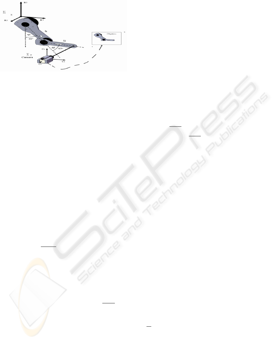
Figure 1: Fixed camera configuration.
represent the robot workspace. A CCD type camera
has a Σ
C
= {C
1
,C
2
,C
3
} Cartesian frame, whose ori-
gin is attached at the intersection of the optical axis
with respect the geometric center of Σ
C
. The descrip-
tion of a point in the camera frame is denoted by x
C
.
The position of the camera frame with respect to Σ
R
is denoted by o
C
= [o
C
1
, o
C
2
, o
C
3
]
T
.
The acquired scene is projected on to the CCD.
To obtain the coordinates of the image at the CCD
plane a perspective transformation is required. We
consider that the camera has a perfect aligned opti-
cal system and free of optical aberrations, therefore
the optical axis intersects at the geometric center of
the CCD plane. Finally the image of the scene on
the CCD is digitalized, transferred to the computer
memory and displayed on the computer screen. We
define a new two dimensional computer image coor-
dinate frame Σ
D
= {u, v}, whose origin is attached to
the upper left corner of the computer screen. There-
fore the vision system model is given by:

u
v

=
λ
λ +x
C
3

α
u
0
0 −α
v

x
C
1
x
C
2

(3)


x
C
1
x
C
2
x
C
3


= R
T
(θ)[x
R
− o
c
R
] (4)
where α
u
> 0, α
v
> 0 are the scale factors in pixels/m,
λ > 0 is the focal length of the camera and
λ
λ+x
C
3
< 0.
2.3 A New Position-based Visual
Servoing Scheme for Fixed-camera
Configuration
In this section, we present the stability analysis for
the position-based visual servoing scheme. The robot
task is specified in the image plane in terms of im-
age feature values corresponding to the relative robot
and object positions. It is assumed that the target re-
sides in the plane R
1
− R
2
, depicted in Figure 2. Let
[u
d
v
d
]
T
be the desired image feature vector which is
assumed to be constant on the computer image frame
Σ
D
. The desired joints q
d
are estimated from inverse
kinematic in function of

u
d
v
d

T
.
The control problem in visual servoing for
fixed-camera configuration consists in to designing
a control law τ in such a way that the actual image
feature

u v

T
reaches the desired image feature

u
d
v
d

T
of the target. The image feature error
is defined as

˜u ˜v

T
=

u
d
− u v
d
− v

T
,
therefore the control aim is to assure that
lim
t→∞

˜q
1
˜q
2

T
=

q
d
1
− q
1
q
d
2
− q
2

T
→ 0.
The control problem is solvable if a joint motion q
d
exists such that

u
d
v
d

=


α
u
λ
λ+x
C
3
0
0
−α
v
λ
λ+x
C
3


R(θ)
T





x
R
1
(q
d
)
x
R
2
(q
d
)

−

o
c
R
1
o
c
R
2





.
(5)
In order to solve the visual servoing control prob-
lem, we present the next control scheme with gravity
compensation:
τ = ∇υ
a
(k
p
,
e
q) − f
v
(k
v
,
˙
q) + g(q) (6)
where
e
q = q
d
− q ∈ R
n
is the position error vector,
q
d
∈ R
n
is the desired joint position vector K
p
∈ R
n×n
is the proportional gain which is a diagonal matrix,
K
v
∈ R
n×n
is a positive definite matrix, also called
derivative gain, ∇υ
a
(k
p
,
e
q) represents the artificial po-
tential energy, being a positive definite function, and
f
v
(k
v
,
˙
q) denotes the damping function, which is a dis-
sipative function, that is, ˙q
T
f
v
(k
v
,
˙
q)> 0.
Proposition. Consider the robot dynamic model (1)
together with the control law (6), then the closed-loop
system is global asymptotically stable, and the visual
positioning aim
lim
t→∞

˜q
1
(t) ˜q
2
(t)

T
= 0 ∈ R
2
is achieved.
Proof: The closed-loop system equation obtained by
combining the robot dynamic model (1) and control
scheme (6) can be written as
d
dt

e
q
˙
q

=


−
˙
q
M(q)
−1

∇υ
a
(k
p
,
e
q)−f
v
(k
v
,
˙
q)
−C(q,
˙
q)
˙
q



(7)
which is an autonomous differential equation, and
the origin of the state space is a equilibrium point.
To carry out the stability analysis of equation (7), the
following Lyapunov function candidate is proposed:
VISUAL SERVOING CONTROLLER FOR ROBOT MANIPULATORS
293

V (
e
q,
˙
q) =
1
2
˙
q
T
M(q)
˙
q +υ
a
(k
p
,
e
q). (8)
The first term of V (
e
q,
˙
q) is a positive definite func-
tion with respect to
˙
q because M(q) is a positive def-
inite matrix. The second one of the Lyapunov func-
tion candidate (8), can be interpreted as a potential
energy induced by the control law, and is also a posi-
tive definite function with respect to the position error
e
q, because the term k
p
is a positive definite matrix.
Therefore, V(
e
q,
˙
q) is both a positive definite and radi-
ally unbounded function.
The time derivative of the Lyapunov function can-
didate (8) along the trajectories of the closed-loop
equation (7), and after some algebra and considering
property 1, can be written as
˙
V (
e
q,
˙
q) =
˙
q
T
M(q)
¨
q −
1
2
˙
q
T
˙
M(q)
˙
q −∇υ
a
(k
p
,
e
q)
T
˙
q
=
˙
q
T
∇υ
a
(k
p
,
e
q) −
˙
q
T
f
v
(k
v
,
˙
q)−C(q,
˙
q)
˙
q
+
1
2
˙
q
T
˙
M(q)
˙
q −∇υ
a
(k
p
,
e
q)
T
˙
q
= −
˙
q
T
f
v
(k
v
,
˙
q) ≤ 0 (9)
which is a negative semidefinite function and
therefore, it is possible to conclude stability in the
equilibrium point. In order to prove local asymp-
totic stability, the autonomous nature of the closed-
loop equation (7) is exploited to apply the LaSalle’s
invariance principle (Khalil, 2002) in the region Ω:
Ω=









e
q
1
e
q
2
˙
q


∈ R
2n
:
˙
V (
e
q,
˙
q) = 0
e
q= 0 ∈ R
n
,
˙
q = 0 ∈ R
n
:
˙
V (
e
q,
˙
q) = 0







(10)
since
˙
V (
e
q,
˙
q) ≤ 0 ∈ Ω, V(
e
q(t),
˙
q(t)) is a decreasing
function of t. V (
e
q,
˙
q) is continuous on the compact set
Ω, it is bounded from below on Ω. For example, it sat-
isfies 0 ≤ V (
e
q(t), (t),
˙
q(t)) ≤ V (
e
q(0),
˙
q(0)). Therefore,
the trivial solution is the only solution of the closed-
loop system (7) restricted to Ω. Consequently it is
concluded that the origin of the state space is locally
asymptotically stable.
2.4 Examples of Application
The purpose of this section is to exploit the methodol-
ogy described above with the objective to derive new
regulators.
We present control scheme with gravity compen-
sation:
τ= K
p
tanh

e
q
1
e
q
2

−K
v
tanh

˙
q
1
˙
q
2

+g(q). (11)
Proof: The closed-loop system equation obtained by
combining the robot dynamic model (1) and control
scheme (7) can be written as
d
dt

e
q
˙
q

=


−
˙
q
M(q)
−1

k
p
tanh(
e
q)−K
v
tanh(
˙
q)
−C(q,
˙
q)
˙
q



(12)
which is an autonomous differential equation, and
the origin of the state space is a equilibrium point. To
carry out the stability analysis of equation (12), the
following Lyapunov function candidate is proposed:
V (
e
q,
˙
q) =
1
2
˙
q
T
M(q)
˙
q+
s
ln

cosh

e
q
1
e
q
2

T
K
p
s
ln

cosh

e
q
1
e
q
2

(13)
The first term of V (
e
q,
˙
q) is a positive definite func-
tion with respect to
˙
q because M(q) is a positive def-
inite matrix. The second one of the Lyapunov func-
tion candidate (13), can be interpreted as a potential
energy induced by the control law, and is also a pos-
itive definite function with respect to position error
e
q, because the term k
p
is a positive definite matrix.
Therefore, V(
e
q,
˙
q) is both a positive definite and radi-
ally unbounded function.
The time derivative of Lyapunov function can-
didate (13) along the trajectories of the closed-loop
equation (12) and after some algebra and considering
property 1, can be written as:
˙
V (
e
q,
˙
q) =
˙
q
T
M(q)
¨
q−
1
2
˙
q
T
˙
M(q)
˙
q −
˙
q
T
K
p
tanh

e
q
1
e
q
2

=
˙
q
T
tanh

e
q
1
e
q
2

−
˙
q
T
K
v
tanh

e
q
1
e
q
2

−C(q,
˙
q)
˙
q+
1
2
˙
q
T
˙
M(q)
˙
q−
˙
q
T
K
p
tanh

e
q
1
e
q
2

= −
˙
q
T
K
v
tanh

˙
q
1
˙
q
2

≤ 0 (14)
A second example from the proposed methodol-
ogy:
τ=K
p
arctan

e
q
1
e
q
2

− K
v
arctan
"
·
q
1
·
q
2
#
+ g(q). (15)
ICINCO 2009 - 6th International Conference on Informatics in Control, Automation and Robotics
294

3 EXPERIMENTAL SET-UP
An experimental system for research of robot control
algorithms has been designed and built at the Uni-
versidad Aut
´
onoma de Puebla, M
´
exico; it is a direct-
drive robot of two degrees of freedom (see Figure 2).
The experimental robot consists of two links made
of 6061 aluminum actuated by brushless direct-drive
servo actuators from Parker Compumotor in order to
drive the joints without gear reduction. Advantages
of this type of direct-drive actuator includes freedom
from backlashes and significantly lower joint friction
compared to actuators composed by gear drives. The
motors used in the robot are listed in Table 1. The
servos are operated in torque mode, so the motors act
as a torque source and they accept an analog volt-
age as a reference of torque signal. Position infor-
mation is obtained from incremental encoders located
on the motors. The standard backwards difference al-
gorithm applied to the joint positions measurements
was used to generate the velocity signals. The manip-
ulator workspace is a circle with a radius of 0.7 m.
Besides position sensors and motor drivers, the robot
also includes a motion control board, manufactured
by Precision MicroDynamics Inc., which is used to
obtain the joint positions. The control algorithm runs
on a Pentium host computer.
Figure 2: Experimental robot.
Table 1: Servo actuators of the experimental robot.
Link Model Torque p/rev
Shoulder DM1050A 50 1,024,000
Elbow DM1004C 4 1,024,000
With reference to our direct-drive robot, only the
gravitational torque is required to implement the new
control scheme (6), which is available in (Malis,
2005):
g(q) =

38.46sin (q
1
) +1.82 sin(q
1
+ q
2
)
1.82sin (q
1
+ q
2
)

[Nm].
(16)
4 EXPERIMENTAL RESULTS
To support our theoretical developments, this Section
presents experimental results of the proposed con-
trollers on a planar robot for the fixed-camera con-
figuration.
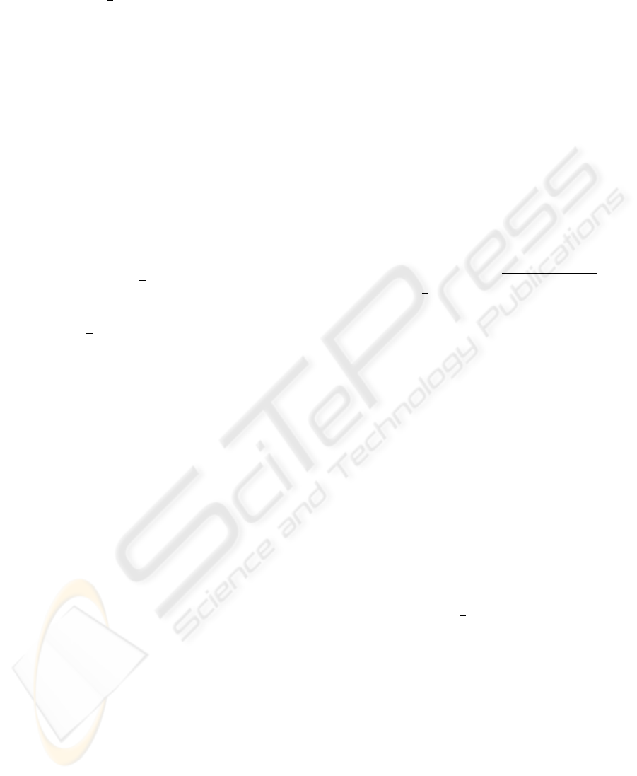
Figure 3: Robot manipulator and vision system.
Three black disks were mounted on the shoulder
joint, elbow joint and end-effector, repestively. A big
black disk for shoulder, a medium black disk on el-
bow, and a small one for the end-effector. The joint
coordinates were estimated from predictable centroid
using inverse kinematics as is shown in Figure (3):
l
1
=
q
(u
2
− u
1
)
2
+ (v
2
− v
1
)
2
(17)
l
2
=
q
(u
3
− u
2
)
2
+ (v
3
− v
2
)
2
(18)
and
q
2
= arccos
(u
3
− u
2
)
2
+ (v
3
− v
2
)
2
− l
2
1
− l
2
2
2l
1
l
2
!
(19)
q
1
=

π
2

− atan

v
2
− v
1
u
2
− u
1

− atan

l
2
sin(q
2
)
l
1
+ l
2
cos(q
2
)

(20)
where l
1
, l
2
represent the link longitude respectively,
u and v are visual information from equations (19)
and (20) using in Figure 3.
The centroids of each disc were selected as ob-
ject feature points. We select in all controllers the
desired position in the image plane as [u
d
v
d
]
T
=
[198 107]
T
[pixels] and the following initial position
[u(0) v(0)]
T
= [50 210]
T
[pixels], this q
1
(0), q
2
(0) =
[0 0]
T
and
˙
q(0) = 0 [degrees/sec]. The evaluated con-
trollers have been written in C language. The sam-
pling rate was executed at 2.5 ms., while the visual
feedback loop was at 33 ms. The CCD camera was
placed in front of the robot and its position with re-
spect to the robot frame Σ
R
was O
R
c
= [0
R
c
1
, 0
R
c
2
, 0
R
c
3
]
T
=
[−0.5, −0.6, −1]
T
meters, the rotation angle θ = 0 de-
grees. We use MATLAB version 2007a, applying, the
VISUAL SERVOING CONTROLLER FOR ROBOT MANIPULATORS
295

SIMULINK module to carry out the imagine process-
ing. The video signal from the CCD-camera has a
resolution of 320x240 pixels in RGB format.
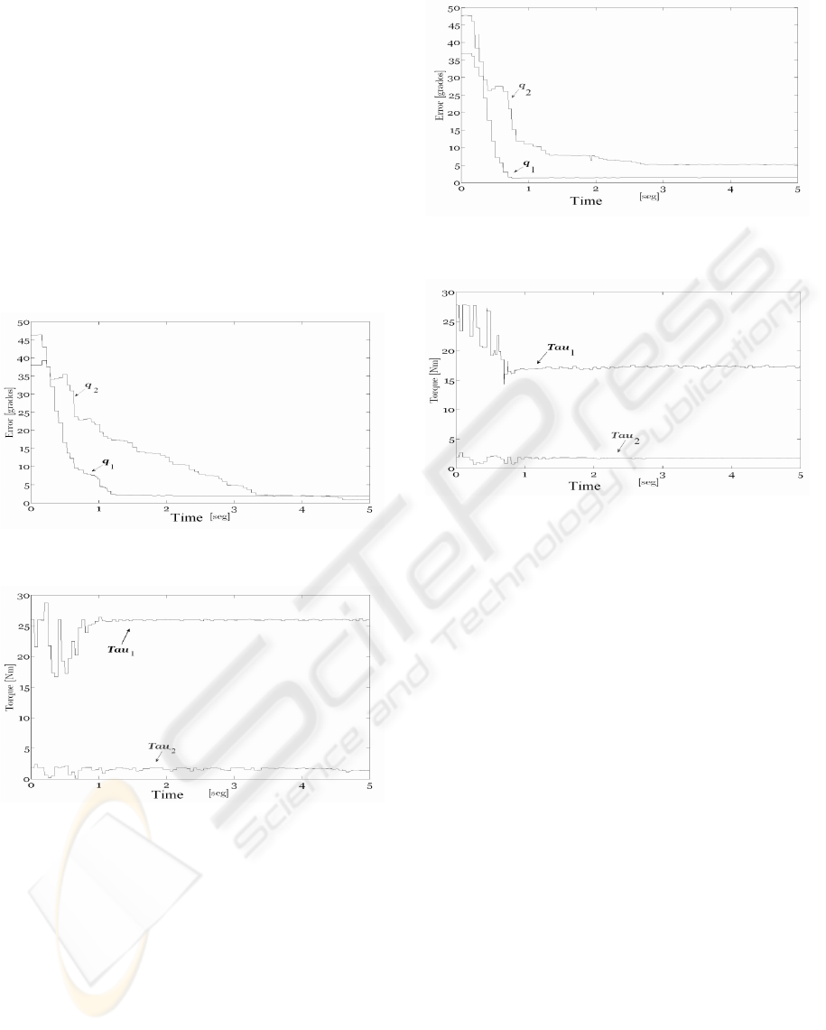
Figures 4 and 5 show the experimental results
of the controller (11), the proportional and deriva-
tive gains were selected as K
p
= diag{26.0, 1.8}
[N], K
v
= diag{12.0, 1.2} [Nm]. respectively and
u
d
= 198 y v
d
= 107. The transient response with
around 3 seconds is fast. The components of the fea-
ture position error tend asymptotically close to zero.
The experimental results for the controller (11) are
shown in Figures (4) and (5). The transient response
was around 3 seconds. The components of the feature
position error tend asymptotically.
Figure 4: Error for controller (11).
Figure 5: Torque for controller tanh.
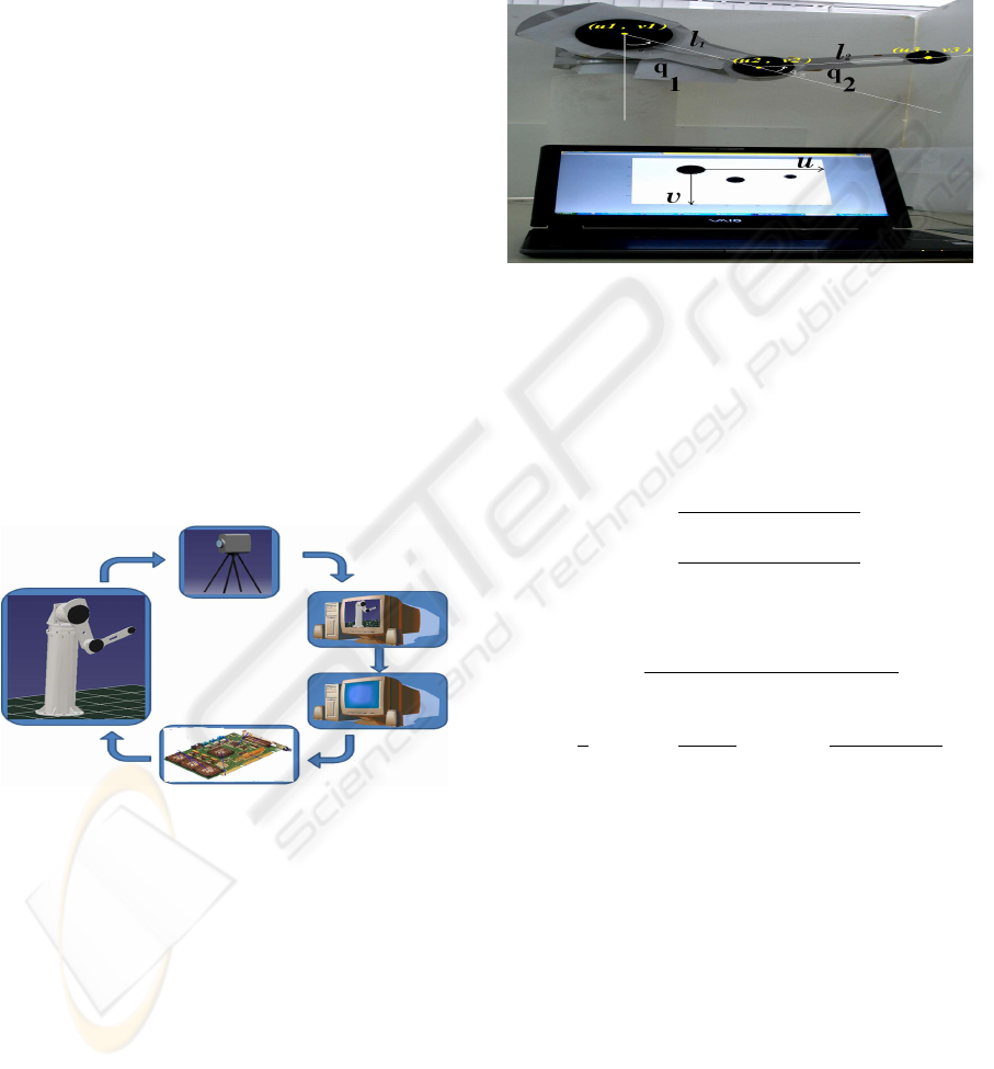
Figures 6 and 7 show the experimental results of
the controller (15). The proportional and derivative
gains were selected as K
p
= diag{17.3, 1.2} [N],
K
v
= diag{6.6, 1.2} [Nm], respectively, and u
d
=
198 y v
d
= 107. The transient response is fast by
around 1 second. The components of the feature posi-
tion error tend asymptotically to a neighborhood close
to zero.
The experimental results for the controller (15) are
shown in Figures 6 and 7. The transient response was
around 1 second. The components of the feature po-
sition error tend asymptotically.
Figure 6: Error for controller (15).
Figure 7: Torque for controller atan.
5 CONCLUSIONS
In this paper we have presented a new methodology
to design position-based visual servoing for planar
robots in fixed-camera configuration. It should be em-
phasized both that the nonlinear robot dynamics and
the vision model have been included in the stability
analysis. The class of controllers are energy-shaping
based, and they are described by control laws com-
posed of the gradient of an artificial potential energy
plus a linear velocity feedback. Experimental results
with a two degrees of freedom planar robot, using
three feature points were presented to illustrate the
performance of the control scheme.
REFERENCES
Hutchinson S., G. D. Hager and P. I. Corke, A Tutorial on
Visual Servo Control. IEEE Trans. on Robotics and
Automation, Vol. 12, No. 5, October 1996, pp. 651-
670.
Hill J. and W. T. Park, Real Time Control of a Robot with a
Mobile Camera. in Proc. 9th ISIR, Washington, D.C.,
Mar. 1979, pp. 233-246.
Weiss L. E., A. C. Sanderson, and C. P. Neuman, Dynamic
sensor-based control of robots with visual feedback.
ICINCO 2009 - 6th International Conference on Informatics in Control, Automation and Robotics
296

in IEEE Journal of Robot. Automat., vol. RA-3, pp.
404-417, Oct. 1987.
Wilson W. J., C. C. Williams, and Graham S. B. Relative
End-Effector Control Using Cartesian Position Based
Visual Servoing. IEEE Transactions on Robotics and
Automation. vol. 12 No. 5, pp. 684-696. October 1996
Kelly R., P. Shirkey and M. W. Spong, Fixed-Camera Visual
Servo Control for Planar Robots. IEEE International
Conference on Robotics and Automation. Minneapo-
lis, Minnesota, April 1996, pp. 2643-2649.
Corke P. I. Visual Control of Robot Manipulators A review.
Visual Servoing, K. Hashimoto, Ed. Singapore: World
Scientific, pp. 1-31, 1993.
Takegaki M. and S. Arimoto, A New Feedback Method
for Dynamic Control of Manipulators. ASME J. Dyn.
Syst. Meas. Control, Vol. 103, 1981, pp. 119-125.
Malis E. and S. Benhimane, A Unified Approach to Visual
Tracking and Servoing. Robotics and Autonomous
Systems, Vol. 52, Issue 1 , 31 July 2005, pp. 39-52.
Conticelli F. and B. Allotta, Nonlinear Controllability and
Stability Analysis of Adaptive Image-Based Systems.
IEEE Trans. on Robotics and Automation, Vol. 17,
No. 2, 2001, pp. 208-214.
Park J. and Y.J. Lee, Robust Visual Servoing for Motion
Control of the Ball on a Plate. Mechatronics, Vol. 13,
Issue 7 , September 2003, pp. 723-738.
Malis E. and P. Rives, Robustness of Image-based Visual
Servoing with Respect to Depth Distribution Errors.
IEEE International Conference on Robotics and Au-
tomation. 2003, pp. 1056-1061.
Spong M. W. and M. Vidyasagar, Robots Dynamics and
Control. John Wiley & Sons, 1989.
Reyes F. and R. Kelly, Experimental Evaluation of Fixed-
Camera Direct Visual Controllers on a Direct-Drive
Robot. IEEE International Conference on Robotics &
Automation. Leuven, Belgium, May 1998, pp. 2327-
2332.
Khalil, H. K. (2002). Nonlinear Systems. Prentice–Hall,
Upper Saddle River, NJ.
Chen J., A. Behal, D. Dawson and Y. Fang, 2.5D Visual Ser-
voing with a Fixed Camera. American Control Con-
ference. 2003, pp. 3442-3447.
Schramm F., G. Morel, A. Micaelli and A. Lottin, Extended-
2D Visual Servoing. IEEE International Conference
on Robotics and Automation. 2004, pp. 267-273.
Reyes F. and R. Kelly (1997). Experimental evaluation of
identification schemes on a direct drive robot. Robot-
ica, Cambridge University Press. Vol. 15, 563–571.
VISUAL SERVOING CONTROLLER FOR ROBOT MANIPULATORS
297