PERFORMANCES IMPROVEMENT AND STABILITY

ANALYSIS OF MULTIMODEL LQ CONTROLLED

VARIABLE-SPEED WIND TURBINES

Nadhira Khezami

1,2

, Xavier Guillaud

and Naceur Benhadj Braiek

LECAP, École Polytechnique de Tunisie, BP 743 – 2078 La Marsa, Tunisia

L2EP, École Centrale de Lille, Cité Scientifique, 59651 Villeneuve d’Ascq Cedex, France

Keywords: LQ controller, Multimodel approach, Global stability, LMI, Lyapunov equations.

Abstract: In this paper, a linear quadratic (LQ) control law combined with a multimodel approach is designed for

variable-speed, variable-pitch wind turbines. The presented technique is based on an optimal control method

in order to improve the system global dynamic. A set of linear local models (sub-models) is then defined for

different operating points corresponding to high wind speeds. Thereafter, a global asymptotic stability

analysis is developed by solving a bilinear matrix inequality (BMI) feasibility problem based on the local

stability of the sub-models.

1 INTRODUCTION

Nowadays, the growth of the utilization of the wind

turbines is more and more important since they are

producing carbon-emission-free electricity. Until

today, only classic control laws, such as P, PI or PID

controllers, are used in the wind turbines. However,

the performance of these controllers is limited by the

high nonlinear characteristics of the wind turbine

and by the appearance of new control objectives

required by the grid-codes; the reason why advanced

control research area is improving every day.

In the first axis of this paper, an LQ controller,

which had been advocated by many researchers, is

designed with a multimodel approach, for pitch

regulated variable speed wind turbines operating at

high wind speeds, in order to guarantee an optimal

behavior for the studied process. However, this

technique still presents some limits to satisfy all the

control objectives especially those concerning the

system global dynamic. This paper aims then to

present an issue for this problem by adding an

exponential term in the quadratic cost function.

The second section deals with the asymptotic

stability analysis of the global system by solving a

set of BMI according to the Lyapunov theorems. In

fact, the stability study is necessary and important to

illustrate the effectiveness of the presented strategy.

Finally, the simulation results realized on Matlab

Simulink are presented and discussed.

2 WIND TURBINE MODELLING

2.1 Wind Turbine Description

The considered wind turbine (Figure 1) is modeled

as two inertias (the generator and the turbine inertias

respectively J

and J

) linked to a flexible shaft with

a mechanical coupling damping coefficient d and a

mechanical coupling stiffness coefficient k. This

model is widely used in the literature (Bianchi et al.,

2004; Camblong et al., 2002).

Figure 1: Wind turbine dynamic model.

where Ω

and Ω

are the turbine and the generator

rotational speeds, T

is the generator torque, T

mec

the drive train mechanical torque and T

aero

is the

torque caught by the wind turbine which is

expressed by:

.(,)

aero p

ρπ

λβ

⋅⋅ ⋅Ω

=⋅

(1)

Khezami N., Guillaud X. and Benhadj Braiek N. (2009).

PERFORMANCES IMPROVEMENT AND STABILITY ANALYSIS OF MULTIMODEL LQ CONTROLLED VARIABLE-SPEED WIND TURBINES.

In Proceedings of the 6th International Conference on Informatics in Control, Automation and Robotics - Intelligent Control Systems and Optimization,

pages 81-88

DOI: 10.5220/0002213100810088

 SciTePress

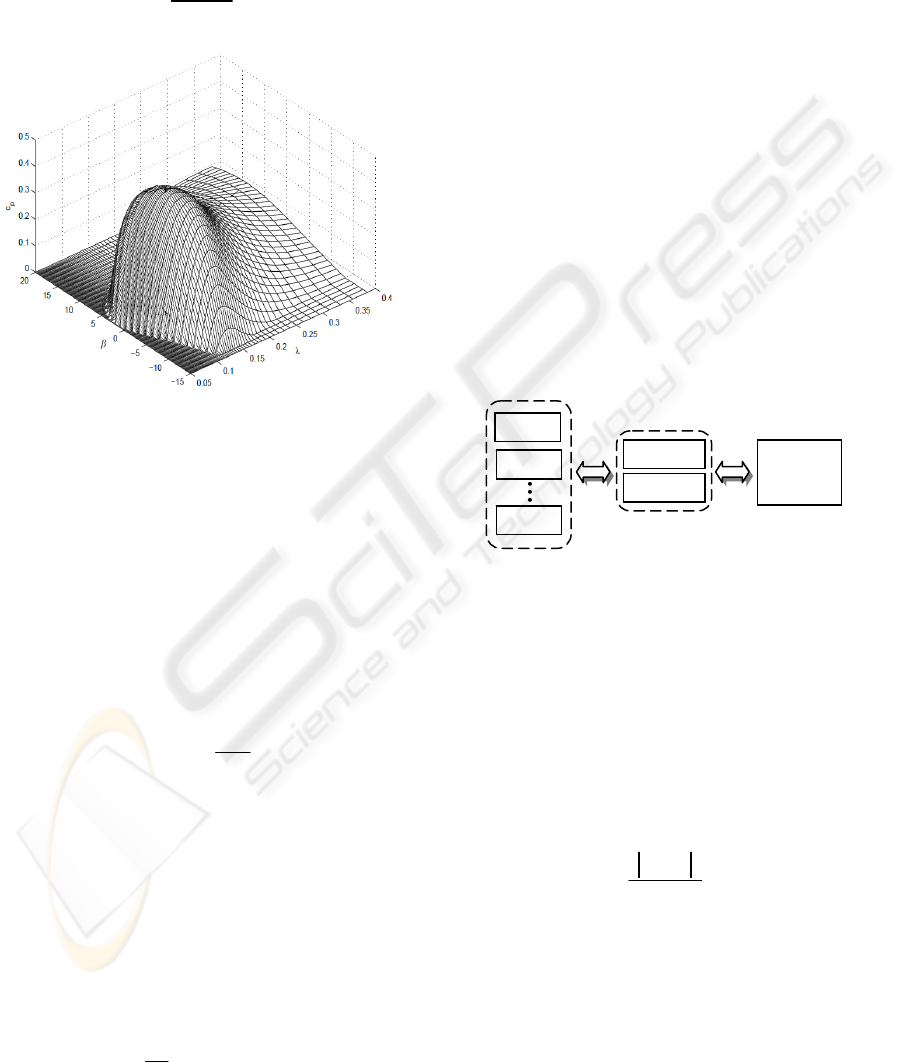
where ρ is the air density and R is the turbine radius.

The power coefficient c

(Figure 2) is a non

linear function of the blade pitch β and the tip speed

ratio λ depending on the wind speed value v and

given by:

Ω⋅

(2)

Figure 2: Power coefficient curves.

The dynamic response of the rotor is given by:

TT aero mec

TTΩ= −



(3)

The generator is driven by the mechanical torque

and braked by the electromagnetic torque. Reported

to the low speed shaft, the characteristic equation is

the following:

ls g ls mec em

TGT

−−

Ω= −



(4)

where G is the gearbox gain and:

².

gls

gls g

−

−Ω =

−=

(5)

And the low speed shaft torque T

mec

results from

the torsion and friction effects due to the difference

between the generator and the rotor speeds

(Boukhezzara et al., 2007). It’s defined by the

following equation reported to the low speed shaft:

.( ) .( )

mec T gls T gls

Tk d

−−

= Ω −Ω + Ω −Ω



(6)

The pitch actuator dynamic is described by a first

order system:

()

ref

βββ

=−



(7)

ref

represents the control value of the blade-pitch

angle β and τ

is the time constant of the pitch

actuator.

2.2 Linearization and State

Representation

The wind turbine is a complex non linear system

presenting several difficulties in study and control. It

seems then more suitable to describe it with a set of

linear local models valid in different operating

points corresponding to different levels of wind

speed values. The principle of this method is used in

several techniques. In this paper, we use the

multimodel approach which was the subject of many

research works (Kardous et al., 2006, 2007).

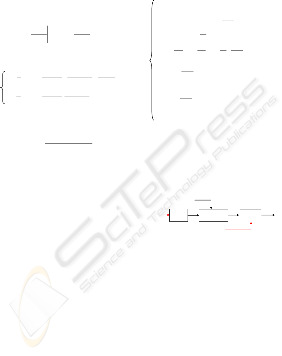
For the studied system, we define a multimodel

base made of four local models. The equivalent

instantaneous model, as described in Figure 3, is

obtained by a fusion of only two valid successive

models. The choice of these models depends on the

wind speed value.

Figure 3: Wind-turbine multimodel description.

The weighting coefficient µ

is the validity value

of the model M

and it can be expressed by:

−

(8)

is a normalized residue measuring the error

between the instantaneous and the valid local model

wind speed values (respectively v and v

). When M

and M

i+1

are the valid models, the residue can be

expressed as:

−

(9)

Thus, the validities satisfy the convex sum, such

that:

µµ

To obtain the local models, the system should be

then linearized around the operating point. The non-

linearity of the system is due to the c

characteristic

which is used in the expression of the aerodynamic

torque. We need then to linearize the expression (1)

M=µ

. M

i+1

. M

i+1

Multimodel base

Equivalent model

Model M

Valid local models

Model M

Model

Model M

i+1

ICINCO 2009 - 6th International Conference on Informatics in Control, Automation and Robotics

of T

aero

around an operating point (o.p) defined by

the wind speed value v

(Bianchi et al., 2007;

Munteanu et al., 2005). We can define:

aero aero

aero T

iTi

∂∂

Δ= ΔΩ+ Δ

∂Ω ∂

=ΔΩ+Δ

(10)

where:

(, )

... . .

(, )

... . .

inom

Tnom inom

T nom

λβ

ρπ

λλ

λβ

ρπ

⎡

⎤

∂

=−

⎢

⎥

Ω∂

⎢

⎥

⎣

⎦

∂

Ω∂

(11)

and:

()

2. .

..².

i nom

p p i nom i nom

T nom aero nom

λβ

ρπ

(12)

The symbol Δ represents the deviation from the

chosen operating point corresponding to (Ω

T_nom

, Ω

ls-nom

, β

i-nom

, T

mec-nom

, T

em-nom

and P

nom

) where: T

em-nom

and T

mec-nom

are respectively the nominal values of

the electromagnetic and the mechanical torques.

Thereafter, the linearization of the non-linear

system expressed in equations (3), (4), (6) and (7)

around an operating point gives a state space

representation of the form below:

{

Ax Bu

yCxDu



(13)

where x, u and y are respectively the state, control

and output vectors defined as:

,and

ref

gls

mec

xy u

−

ΔΩ

⎡⎤

⎢⎥

ΔΩ

⎡⎤

ΔΩ

⎡⎤

== =

⎢⎥

⎣⎦

⎢⎥

⎣⎦

(14)

Notice that P=T

.Ω

designates the generated

electrical power. This leads to write around an

operating point:

()

.. .

em nom g ls em g ls nom

PGT T

−−

Δ= ΔΩ +Δ Ω

(15)

Hence, A

, B

, C

and D

, which are respectively

the state, input, output and feedthrough matrices, are

defined as follows:

000

00 0

1000

0. 00

and

TT T

gls

TTTgls

gls

em nom

gls

glsnom

JJ J

ad db

kk d

JJJJ

−

⎛⎞

−

⎜⎟

−

⎜⎟

⎛⎞

⎜⎟

+− −+

⎜⎟

⎝⎠

⎛⎞

⎜⎟

−

⎜⎟

⎛⎞

⎜⎟

⎝⎠

⎜⎟

⎝⎠

⎛⎞

⎜⎟

⎝⎠

(16)

3 CONTROLLER DESIGN

The control task is based on the objective of

regulating the rotor rotational speed and the

generated power by acting on two control variables:

the electromagnetic torque T

and the regulating

pitch angle β

ref

Pitch

actuator

Aerodynamic

ste



Electrical

ste m



el ec

wind



Figure 4: Wind turbine block diagram.

The LQ control strategy had been advocated by

many research works (Boukhezzara et al., 2007;

Khezami et al., 2009; Poulsen et al., 2005;

Hammerum et al., 2007; Cutululis et al., 2006). This

technique presents a good compromise between the

performances optimization and the minimization of

the control signals by the use of a quadratic cost

function. However, it also presents the disadvantage

of the non possibility of controlling the global

system dynamic. In this paper, a solution that can

partially solve this problem is presented.

This controller aims to minimize the following

quadratic criterion J :

()

.. .. .

TT t

yQy uRue dt

+∞

∫

(17)

where Q and R are diagonal positive definite

matrices.

PERFORMANCES IMPROVEMENT AND STABILITY ANALYSIS OF MULTIMODEL LQ CONTROLLED

VARIABLE-SPEED WIND TURBINES

The term y

.Q.y expresses the performances

optimization, the term u

.R.u expresses the

minimization of the control signals and the term e

2αt

allows the performances improvement of the classic

quadratic criterion. It leads to the placement of the

system poles on the left of -α.

The criterion can be rewritten as follows with an

input-state cross term:

()

.. 2... ...

TTTt

xQx xNu uRue dt

+∞

=++

∫

(18)

where Q

, R

and N are defined as :

QCQC

RRDQD

NCQD

⎧

⎪

⎨

⎪

⎩

(19)

For this criterion, the optimal gain can be

calculated from the following Riccati equation:

11 1

.. (. )..(. )

.( . )

TTT

iii i

ALLA LBNRBLN

AA I

KRBLN

αα

−

⎧

+−+ +

⎪

⎨

⎪

⎩

(20)

where I is the identity matrix.

Since the dynamic of the pitch actuator should

not be changed, the controller is designed in two

steps. In the first step, we consider the blade pitch

angle β and the electromagnetic torque T

as control

variables instead of β

ref

and T

. The state

representation becomes then:

{

1i11i11

i1 1 i1 1

Ax Bu

yCx Du



(21)

where:

()

,and

and

1gls 1

mec

gls

TTgls

gls

Tgls

em nom

xyu

A00

kkd

JJJ

100

0GT 0

−

⎡⎤

ΔΩ

⎡⎤

⎢⎥

=ΔΩ = =

⎢⎥

⎣⎦

⎢⎥

⎣⎦

⎛⎞

⎜⎟

−

⎜⎟

⎛⎞

⎜⎟

+−−+

⎜⎟

⎝⎠

⎛⎞

⎜⎟

=−

⎜⎟

⎝⎠

()

(22)

From this representation, the optimal gain

i1 Tem

⎡

⎤

⎢

⎥

⎢

⎥

⎣

⎦

is calculated such that:

1i11

uKx

⎡⎤

==−

⎢⎥

⎣⎦

(23)

The relation (23) leads to the following optimal

control law using the global state vector as shown in

Figure 5:

iref

iTem

uKx

=−

⎧

⎪

⎡

⎤

⎨

⎢

⎥

⎪

⎢

⎥

⎣

⎦

⎩

(24)

with:

(

)

_ 1_ 1_11 1_1_2

1_ 1_ 1_ 1

_1_1

... ...

.. . .

iref i i i i i

i i Tem i Tem

i Tem i Tem

KKKATKBT

KB K T

KKT

βββββββ

ββ

ττ

⎧

++ −

⎪

⎨

⎪

⎩

(25)

and:

[]

1_ 1_ 1

1000

0100

0001

0010

iiTemi

BB B

⎧

⎡⎤

⎣⎦

⎪

⎡⎤

⎪

⎢⎥

⎨

⎢⎥

⎪

⎣⎦

⎪

⎩

(26)

Figure 5: The LQ controller design.

4 STABILITY STUDY

The quantum advance in stability theory that

allowed one the analysis of arbitrary differential

equations is due to Lyapunov, who introduced the

ls−

mec

em nom

−

TΔ

Tnom−

ls nom−−

i nom

−

i nom

−

ref

ΔΩ

ls−

ΔΩ

mec

TΔ

−

()

ii1

wind

vvv

mec nom

−

ICINCO 2009 - 6th International Conference on Informatics in Control, Automation and Robotics

0 5 10 15 20 25 30 35 40 45 50

1.87

1.88

1.89

1.9

1.91

1.92

time (s)

rot at ional speed (rad/ s)

local model

improved LQ

classsic LQ

0 5 10 15 20 25 30 35 40 45 50

1.86

1.88

1.9

1.92

local model

time (s)

rot ati onal speed (rad/ s)

0 5 10 15 20 25 30 35 40 45 50

1.84

1.86

1.88

1.9

local model

time (s)

rot at ional speed (rad/ s)

classic LQ

improved LQ

classic LQ

0 5 10 15 20 25 30 35 40 45 50

1.84

1.86

1.88

1.9

1.92

local model

time (s)

rot at ional speed (rad/ s)

classic LQ

improved LQ

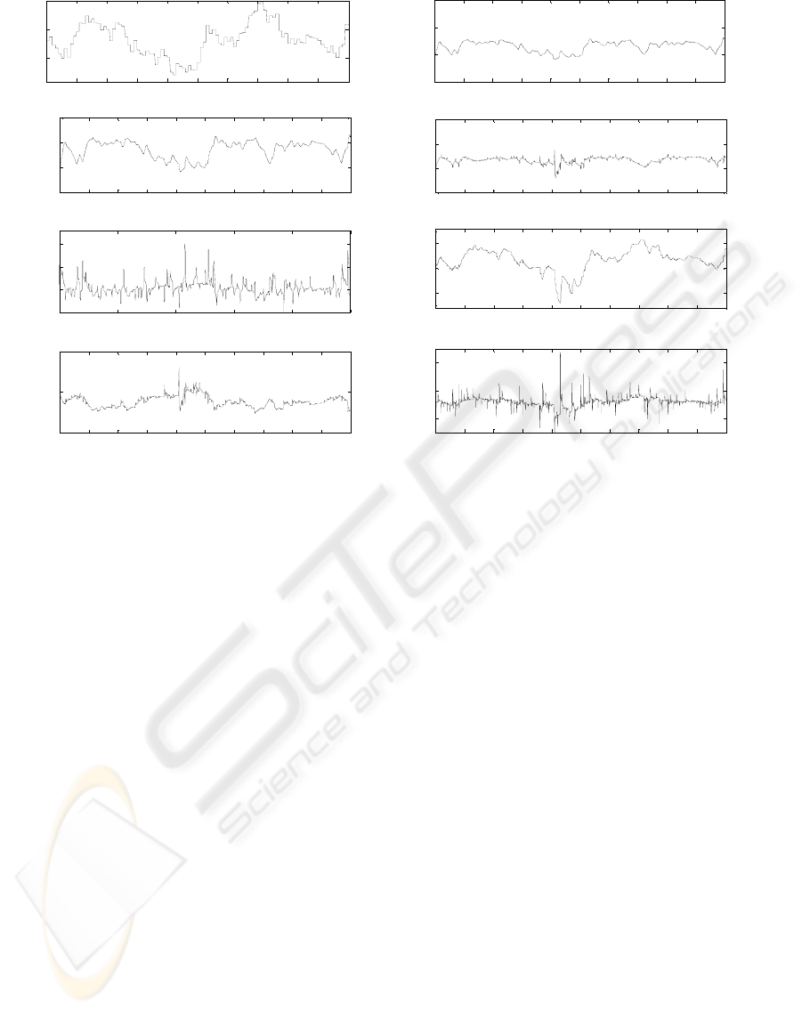
Figure 6: Comparison simulation between classic and improved LQ control laws.

basic idea and the definitions of stability that are in

use today. The concept of Lyapunov stability plays

an important role in control and system theory.

As we define a global model

M by fusion of two

successive local models

and M

i+1

, the

characteristic matrices of the system (13) can be

obtained by:

ikkkk

AA A

BB B

CC C

DD D

μμ

⎧

⎪

⎨

⎪

⎩

(27)

The input vector is calculated by:

()

...

kk k k

uKKx

μμ

=− +

(28)

Hereafter, the state vector can be represented as:

()

.. . .

.. 2. .. .

ij i i j

ij ji

iii ij

iji

xABKx

Gx x

μμ

μμμ

=−

⎛⎞

⎜⎟

⎝⎠

∑∑



(29)

where:

ij i i j

GABK=−

To study the global asymptotic stability of the

above system supplied by the multimodel LQ

control, the first necessity is to analyze the stability

of every local model. A

s we focus here especially on

the closed-loop system, the criterion of stabilization

consists then in finding, for a local model

, a

positive definite matrix

P that satisfies the following

LMI (Chedli, 2002; Liberzon and Morse, 1999):

..0

ii ii

GP PG+<

(30)

In the case of the multimodel systems, an extra

condition is to add to the LMI (30) in order to

guarantee the global stability (Chedli, 2002;

Liberzon and Morse, 1999; Kardous

et al., 2003)

and it consists in:

..0,

ij ij

QP PQ i j

(31)

where

ij ji

And in our case, only two successive local

models are valid at a time, which means that this

condition will be considered for i=1 to 3 and j=i+1.

5 SIMULTATION RESULTS

The proposed control approach and the stability

analysis of the controlled system have been

illustrated through simulations on Matlab Simulink.

The simulated wind turbine parameters are

presented in Table 1.

To calculate the linearization coefficients a

and

, the following c

empiric expression relative to

2MW wind turbines is used:

0.16

0.4 0.5

0.18 6.8 0.115

0.4 0.5

−

⎛⎞

=× −− ×

⎜⎟

⎝⎠

(32)

Table 1: Wind turbine parameter values.

Parameters

Values

Air density ρ 1,22 Kg/m

Turbine radius R 40m

Nominal power P

nom

2MW

Nominal speed Ω

-nom

18 rpm

Optimal power

coefficient

p-opt

0.4775

Optimal speed ratio λ

Gearbox gain G 92.6

Turbine inertia JT 4.9×10

N.m.s²

Generator inertia Jg 0.9×10

N.m.s²

Mechanical coupling

damping coefficient

d 3.5×10

N.m

-1

Mechanical coupling

stiffness coefficient

k 114×10

N.m

-1

PERFORMANCES IMPROVEMENT AND STABILITY ANALYSIS OF MULTIMODEL LQ CONTROLLED

VARIABLE-SPEED WIND TURBINES

Table 2 describes the four local models multimodel

base used for the simulations.

Table 2: Multimodel base parameters.

Local model

Wind speed

vi (m/s)

Pitch angle

i-nom

(°)

M1 11.6 1.1

M2 14 8

M3 17 11.1

M4 25 15.4

From this base, four optimal gains are calculated.

And thus, the stability feasibility problem

consists in solving 8 LMI as shown after:

0(1 )

. . 0, 1..4 (4 )

..0,1..3, 1(3)

ii ii

ij ij

PLMI

GPPG i LMI

QP PQ i j i LMI

⎧

⎪

+<=

⎨

⎪

+<= =+

⎩

(33)

The simulation leads to the following result:

8.848 8.335 0.008 0.298

8.335 8.101 0.007 0.258

0.53 0.523 0.026 0.001

0.298 0.258 0.001 0.084

−−

⎛⎞

⎜⎟

−−

⎜⎟

−−

⎜⎟

−−

⎝⎠

Finding this positive definite matrix P is a

sufficient condition proving the global stability of

the control technique presented above.

For the simulations, we had chosen to place the

closed loop poles for the local models at the left of

-α=-0.5. This gives the following poles for each

local model:

 1

local model:

1.032 12.24

1.069

−+

⎡⎤

−−

⎢⎥

−

⎢⎥

−

⎣⎦

 2

local model:

1.032 12.24

1.06

−+

⎡⎤

−−

⎢⎥

−

⎢⎥

−

⎣⎦

 3

local model:

1.033 12.24

1.049

−+

⎡⎤

−−

⎢⎥

−

⎢⎥

−

⎣⎦

 4

local model:

1.037 12.24

1.046

−+

⎡⎤

−−

⎢⎥

−

⎢⎥

−

⎣⎦

Thus, we can see that the pitch system pole (-1)

is invariant for the four local models, and that all the

other poles have their real parts less than –α.

To test the performance of this control strategy, a

series of simulation for several wind steps has been

performed to show the improvement of the studied

controller against a classic multimodel LQ controller

(Khezami et al., 2009).

The Figure 6 presents a comparison simulation

between the two control laws. For this simulation,

only the turbine rotational speed response for a wind

step of 0.5 m/s is presented for the four local

models.

The local models poles for the classic LQ

strategy have the following values:

 1

local model:

0.346 12.25

1.162 + 0.868

1.162 0.868

−+

⎡

⎤

−−

⎢

⎥

⎢

⎥

−

⎢

⎥

−−

⎣

⎦

 2

local model:

1.2 12.401

2.693 + 2.013

2.693 2.0128

−+

⎡⎤

−−

⎢⎥

−

⎢⎥

−−

⎣⎦

 3

local model:

1.62 12.587

3.417+2.287

3.417 2.287

−+

⎡

⎤

−−

⎢

⎥

⎢

⎥

−

⎢

⎥

−−

⎣

⎦

 4

local model:

2.148 12.845

4.108+2.418

4.1081 2.418i

−+

⎡⎤

−−

⎢⎥

−

⎢⎥

−−

⎣⎦

In the comparison between both strategies, the

system response for the proposed controller has

indeed kept almost the same response time (about

4s), unlike the case with the classic LQ where the

response times are varying from 12s for the 1

local

model to 2s for the 4

local model.

Compared to the proposed strategy, the classic

multimodel LQ control law shows responses with a

more oscillating transient mode.

The improvements of the multimodel LQ

controller consist in a more damped oscillatory

mode and a faster dynamic than the classical control

mode with an almost fixed response time for all the

local models.

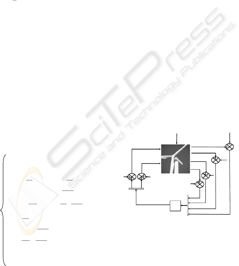
The simulation of the system with the proposed

control strategy for a variable wind speed between

12m/s and 25m/s leads to the results presented in the

curves of Figure 7.

The Figure 7 (a) illustrates a realistic aspect of

the wind speed as described in a method elaborated

by C. Nichita in (Nichita et al., 2003). From this

aspect, the controller allowed a good regulation of

the generated electrical power (Figure 7 (d)) and the

rotation speeds of both the rotor (Figure 7 (b)) and

the generator (Figure 7 (c)) around their rated values

with taking into account the fatigue damage since

the mechanical torque (Figure 7 (e)) maintains an

almost constant value which thereby leads to have

alleviated mechanical loads.

The variations of the electromagnetic torque

presented in Figure 7 (g) are smooth. However, the

price paid for these performances is shown in Figure

7 (h) by a large activity of the pitch actuator.

ICINCO 2009 - 6th International Conference on Informatics in Control, Automation and Robotics

0 10 20 30 40 50 60 70 80 90 100

time (s)

Wind speed (m/s)

0 10 20 30 40 50 60 70 80 90 100

1.8

1.9

2.1

time (s)

Rotor speed (rad/s)

0 10 20 30 40 50 60 70 80 90 100

170

175

180

185

time (s)

Generator speed (rad/s)

0 10 20 30 40 50 60 70 80 90 100

1.9

2.1

2.2

x 10

time (s)

Generated power (W)

0 20 40 60 80 100

1.05

1.1

1.15

x 10

time (s)

Mechani cal t orque (Nm)

0 10 20 30 40 50 60 70 80 90 100

time (s)

Pitch angle (°)

0 10 20 30 40 50 60 70 80 90 100

1.1

1.15

1.2

x 10

time (s)

Electromagnetic torque (Nm)

0 10 20 30 40 50 60 70 80 90 100

time (s)

Control pitch angle (°)

Figure 7: Variation of the system variables.

6 CONCLUSIONS

This paper dealt with a technique of designing a

multimodel LQ regulator allowing to partially

control the process global dynamic, and with a study

of the global asymptotic stability of the controller by

means of a set of LMI. The proposed strategy

presented a compromise between different control

objectives: optimizing the performances of the

different system variables especially generating an

electrical power of a good quality, minimizing the

control efforts, alleviating the drive train dynamic

loads and controlling the global dynamic of the

studied process. The simulations results showed

good performances of the controller with acceptable

mechanical stress. But, satisfying such a trade-off

between all these objectives is indeed difficult and

the cost is however some high forces on the pitch

actuator. These effects brought more challenges in

the system analysis to improve the obtained results

in order to control actively the system dynamic and

to totally damp the oscillatory mode.

REFERENCES

Bianchi, F. D., Mantz, R. J. and Christiansen, C. F., 2004,

Control of Variable-speed Wind Turbines by LPV

Gain Scheduling. In Wind Energy, vol. 7, issue 1, pp:1-8.

Camblong, H., Rodriguez, M., Puiggali, J. R. and Abad,

A., 2002, Comparison of different control strategies to

study power quality in a variable-speed wind turbine.

In 1

World wind Energy Conference Proceeding,

Berlin.

Boukhezzara, B., Lupua, L., Siguerdidjanea, H. and Hand,

M., 2007. Multivariable control strategy for variable

speed, variable pitch wind turbines. In Science Direct,

Renewable Energy, vol. 32, pp: 1273–1287.

Kardous, Z. , Benhadj Braiek, N. and Al Kamel, A., 2006.

On the multimodel stabilization control of uncertain

systems – Part 1, In International Scientific IFNA-ANS

Journal: Problems on Nonlinear Analysis in

Engineering Systems, No 2.

Kardous, Z., Benhadj Braiek, N. and Al Kamel, A., 2007.

On the multimodel stabilization control of uncertain

systems – Part 2. In Int. J. of Problems of Nonlinear

Analysis in Engineering Systems, No.1(27), pp: 76-87,

vol. 13.

Bianchi, F. D., De Battista, H. and Mantz, R. J., 2007.

Wind turbine control systems: principles, modeling

and gain scheduling design, Springer-Verlag. London,

edition.

Munteanu, I., Bratcu, A. I., Cultululis, N. A. and Ceanga,

E., 2005. A two loop optimal control of flexible drive

train variable speed wind power systems, 16

Triennial World Congress-IFAC, Prague.

Khezami, N., Guillaud, X., and Benhadj Braiek, N., 2009.

Multimodel LQ controller design for variable-speed

and variable pitch wind turbines at high wind speeds.

In IEEE International Multi-conference on Systems,

Signals and Devices, Djerba.

(a)

(b)

(c)

(d)

(e) (f)

(g)

(h)

PERFORMANCES IMPROVEMENT AND STABILITY ANALYSIS OF MULTIMODEL LQ CONTROLLED

VARIABLE-SPEED WIND TURBINES

Poulsen, N. K., Larsen, T. J., and Hansen, M. H., 2005.

Comparison between a PI and LQ-regulation for a 2

MW wind turbine. Risø National Laboratory-I-2320.

Hammerum, K., Brath1, P. and Poulsen, N. K., 2007. A

fatigue approach to wind turbine control. In Journal of

Physics: Conference Series 75.

Cutululis, N. A., Bindner, H., Munteanu, I., Bratcu, A.,

Ceanga, E., and Soerensen, P., 2006. LQ Optimal

Control of Wind Turbines in Hybrid Power Systems.

In European Wind Energy Conference and Exhibition,

Athens.

Chedli, M., 2002. Stabilité et commande de systems

décrits par des multimodèles. PhD thesis, Institut

National Polytechnique de Lorraine.

Liberzon, D. and Morse, A. S., 1999. Basic problems in

stability and design of switched systems. In IEEE

Control Systems Magazine, vol. 19, pp: 59-70.

Kardous, Z., Elkamel, A., Benhadj Braiek, N. and Borne,

P., 2003. On the quadratic stabilization in discrete

multimodel control. In IEEE Conference on Control

Applications, vol.2, pp: 1398-1403.

Nichita, C., Luca, D. and Dakyo, B., 2003. Méthodes de

simulation de la vitesse du vent. In Decentralized

energy seminar, Toulouse.

This work was supported by the CMCU project number:

08G1120

ICINCO 2009 - 6th International Conference on Informatics in Control, Automation and Robotics