IFT-BASED PI-FUZZY CONTROLLERS
Signal Processing and Implementation
Radu-Emil Precup, Mircea-Bogdan Rădac, Stefan Preitl
Dept. of Automation and Appl. Inf., “Politehnica” University of Timisoara
Bd. V. Parvan 2, 300223 Timisoara, Romania
Marius-Lucian Tomescu
Fac. of Computer Sci., “Aurel Vlaicu” University of Arad, Complex Univ. M
Str. Elena Dragoi 2, 310330 Arad, Romania
Emil M. Petriu
School of Information Technology and Eng., University of Ottawa
800 King Edward, Ottawa, ON, K1N 6N5 Canada
Adrian Sebastian Paul
Dept. of Automation and Appl. Inf., “Politehnica” University of Timisoara
Bd. V. Parvan 2, 300223 Timisoara, Romania
Keywords: Iterative Feedback Tuning, PI-fuzzy controllers, Stability analysis.
Abstract: New Takagi-Sugeno PI-fuzzy controllers (PI-FCs) are suggested in this paper. The PI-FC design is based on
the optimization of PI controllers in terms of the Iterative Feedback Tuning (IFT) approach. Next the
parameters of the PI controllers are mapped onto the parameters of the Takagi-Sugeno PI-FCs in terms of
the modal equivalence principle. An attractive design method is derived to support the implementation of
low-cost PI-FCs. The design is enabled by a stability analysis theorem based on Lyapunov’s theorem for
time-varying systems. The theoretical approaches are validated by a case study corresponding to the
position control of a servo system. Real-time experimental results are included.
1 INTRODUCTION
The design of control systems (CSs) making use of
measurement data is successful in many industrial
applications without models available for the
controlled process. The time-consuming design of
those models can be avoided. Fuzzy control is an
alternative when very good steady-state and
dynamic CS performance indices can be guaranteed.
The systematic design of fuzzy controllers must be
assisted by the analysis of the fuzzy CS structural
properties i.e. stability, controllability, parametric
sensitivity and robustness (Sala et al., 2005; Kovačić
and Bogdan, 2006; Blažič and Škrjanc, 2007).
Iterative Feedback Tuning (IFT) is a gradient-
based approach, based on input-output data recorded
from the closed-loop system (Hjalmarsson et al.,
1998). The performance specifications are expressed
in terms of objective functions in appropriate
optimization problems. Those problems can be
solved by iterative gradient-based minimization
implemented as IFT algorithms. IFT makes use of
closed-loop experimental data to calculate the
estimates of the gradients of the objective functions.
Several experiments are done per iteration and the
updated controller parameters are calculated based
on the input-output data. So the IFT belongs to the
direct data-based offline-adaptive controller designs.
The combination of IFT and fuzzy control leads
207
Precup R., R
ˇ
adac M., Preitl S., Tomescu M., Petriu E. and Paul A. (2009).
IFT-BASED PI-FUZZY CONTROLLERS - Signal Processing and Implementation.
In Proceedings of the 6th International Conference on Informatics in Control, Automation and Robotics - Intelligent Control Systems and Optimization,
pages 207-212
DOI: 10.5220/0002204502070212
Copyright
c
 SciTePress

to the convenient performance enhancement of
fuzzy CSs after their initial tuning (Precup et al.,
2008). The first contribution of the paper concerns
the modification of the second experiment specific
to IFT to be overlapped over the normal CS
operation. Several useful remarks are introduced in
relation with the signal processing and
implementation of the IFT algorithms. The second
contribution is a new design method of low-cost
Takagi-Sugeno PI-FCs which is based on mapping
the results from the linear case onto the fuzzy one in
terms of the modal equivalence principle (Galichet
and Foulloy, 1995). The third contribution is a
stability analysis theorem based on Lyapunov’s
theorem for time-varying systems derived from
(Slotine and Li, 1991) to support the PI-FC design.
The paper is organized as follows. Section 2
discusses the signal processing and implementation
aspects regarding the IFT algorithm. Next, Section 3
presents the new design method for a class of
Takagi-Sugeno PI-FCs. Section 4 addresses a case
study associated with low-cost implementations of
DC drive servo system position CSs. The
conclusions are presented in Section 5.
2 SIGNAL PROCESSING AND
IMPLEMENTATION ASPECTS
IN IFT ALGORITHMS
The IFT-based CS structure is presented in Figure 1,
where: r – the reference input, d – the disturbance
input,
y
r
e −=
– the control error, u – the control
signal, ρ – the parameters vector having the
controller tuning parameters as its components, C(ρ)
– the transfer function of the linear controller, a PI
one, here to be replaced by the PI-FC, in order to
improve the CS performance indices, F – the
transfer function of the reference model that
prescribes the desired behaviour to be exhibited by
the closed-loop system, P – the transfer function of
the controlled process, y – the controlled output, y
d
–
the desired output produced by the reference model,
d
yyy −=δ
– the model tracking error, and IFT – the
Iterative Feedback Tuning algorithm, i – the input
vector to set the performance specifications.
Figure 1: CS structure with IFT.
The operational variable in the transfer functions
has been omitted for the sake of simplicity. However
that variable will be mentioned in the sequel in the
well accepted notation s for continuous-time systems
and z for discrete-time ones to improve the clarity of
the presentation when needed. That is also the
reason for inserting or removing the argument ρ.
The controller parameterization is such that the
transfer function C(ρ) is differentiable with respect
to ρ. The controller must ensure an initially
stabilized CS. The initial controller tuning affects
the convergence of the iterative process.
The accepted expression of the objective
function J(ρ) is
∑
=
δ=
N
k
kyNJ
1
2
)],([)/5.0()( ρρ
,
(1)
where: N – the number of samples setting the length
of each experiment. A typical objective is to find a
parameters vector
*
ρ
to minimize J(ρ) and make the
error δy tend to zero by the optimization problem
)(
minarg
*
ρρ
ρ
J
SD∈
=
,
(2)
where several constraints can be imposed regarding
the controlled process or the closed-loop CS. The
most important constraint accepted in this paper
concerns the necessity of stable CSs, and SD stands
for the stability domain. Other variables including
the control signal can be used. That requires
additional signal processing and increased cost.
The IFT algorithms solve the optimization
problem (2) by means of numerical optimization
techniques. Newton’s method is popular in IFT since
it can be treated independently of the difficulties
inherent to the model-based techniques. It evaluates
repeatedly a new solution based on a point of the
function and its approximate derivative. The
mathematical formulation is the following update
law to calculate the next set of parameters
1+i
ρ
:
ICINCO 2009 - 6th International Conference on Informatics in Control, Automation and Robotics
208

)]([)(
11 iiiii
J
est ρ
ρ
Rρρ
∂
∂
γ−=
−+
,
(3)
where: i – the index of current iteration,
)]([
i
J
est ρ
ρ∂
∂
– the estimate of the gradient vector,
i
γ
– the step
size,
0
ρ
– the initial guess of the tuning parameters,
and R
i
– a regular positive definite matrix. R
i
can be
the Hessian or the identity matrix to simplify the
signal processing.
Differentiating (1), the gradient becomes
)],(),([)/1()(
1
i
N
k
ii
k
y
kyN
J
ρ
ρ
ρρ
ρ ∂
δ∂
δ=
∂
∂
∑
=
.
(4)
To calculate the general expressions of the gradient
of the output error it is necessary to make use of the
information obtained from the closed-loop system.
The sensitivity function S and the complementary
sensitivity function T must be expressed:
].)(1/[)()(1)(
],)(1/[1)(
PCPCST
PCS
ρρρρ
ρρ
+=−=
+=
(5)
The differentiation of
)(ρyδ
making use of (5) and
Figure 1 leads to the gradient of
)(ρyδ
:
)(
)(
)(
)(
1
)( yrT
C
C
y
−
∂
∂
⋅=
∂
δ∂
ρρ
ρρ
ρ
ρ
.
(6)
To obtain the estimate of the gradient of the
model tracking error use is made of two experiments
per iteration for the PI controllers. In the first
experiment, the normal one, use is made of Figure 1,
the reference input r
1
is applied to the CS and the
controlled output y
1
is measured. In the second
experiment, the gradient one, the control error of the
first experiment
111
yre
−
=
is applied as the
reference input r
2
(Hjalmarsson et al., 1998) and the
controlled output y
2
is measured. That processing is
far away from the normal CS operation. Therefore a
new gradient experiment is suggested here where the
reference input r
2
is applied and the signal e
1
is
injected after the control signal. That can be
expressed as the experimental scheme for the
gradient experiment illustrated in Figure 2 where the
blocks F and IFT have been dropped out.
Figure 2: Experimental scheme for gradient experiment.
Accepting the lower subscript pointing out the
index of the current experiment, the reference input
and controlled output in the normal experiment are
111
)(
)()( ,
dSrTyrr ρρρ +
=
=
.
(7)
For the gradient experiment, making use of the
Figure 2, the results are
,
)(
)](]}()(1/[{
)()( ,
211
222
dSyrPCP
rTyrKr
ρρρ
ρρ
+−++
+
=
=
(8)
where the gain K has been inserted to show the
proportional reference inputs in the two experiments.
Next (7) is multiplied by K, extracted from (8), the
relationship (6) is used and the result becomes
).,(
/)]( )()[()],(
),([
),(
),(
1
121
2
1
i
ii
iii
qC
kdKkdSkyK
ky
q
C
k
y
ρ
ρρ
ρρ
ρ
ρ
ρ
−
−
−−−
−
∂
∂
=
∂
δ
∂
(9)
The second term in the right-hand side of (9)
depends on the disturbance inputs, it affects the
gradient, so it should be alleviated. Neglecting that
term the estimate of the gradient of δy is evaluated:
)].,(
),([
),(
)],([
1
2
1
i
iii
kyK
ky
q
C
k
y
est
ρ
ρρ
ρ
ρ
ρ
−
−
∂
∂
=
∂
δ
∂
−
(10)
The alleviation of the second term in the right-
hand side of (9) can be done by the proper initial
tuning of the controller parameters because
)(
i
S ρ
plays the role of filter. That term can lead to shifted
estimates with negative effects on the convergence.
A similar approach (Hildebrand et al., 2005) is
characterized by an additional prefilter designed as
solution to optimization problems. That filter is not
introduced here to simplify the signal processing
accepting that K=1. The role of
0
ρ
is highlighted
from that point of view.
Summarizing all signal processing aspects
mentioned before in the linear case, one iteration in
the IFT algorithm consists of the following steps.
Step 0. Set
0
ρ
.
Step 1. The two experiments are done making
use of the CS structures presented in Figure 1 and
Figure 2 and the outputs y
1
and y
2
are measured.
Step 2. The output of the reference model is
generated, y
d
, and the output error δy is calculated.
Step 3. The estimate of gradient of J is calculated
according to (4) and (10).
Step 4. The next set of parameters
1+i
ρ
is
calculated in terms of the update law (3).
IFT-BASED PI-FUZZY CONTROLLERS - Signal Processing and Implementation
209

3 DESIGN OF TAKAGI-SUGENO
PI-FUZZY CONTROLLERS
The Takagi-Sugeno PI-FC is a discrete-time
controller built around the two inputs-single output
fuzzy controller (TISO-FC), Figure 3, where
Δe(k)=e(k)–e(k–1) and Δu(k)=u(k)–u(k–1) is the
increment of control error and signal, respectively.
The fuzzification is done by the membership
functions presented in Figure 4, the inference engine
employs the MAX and MIN operators assisted by
the rule base presented in Table 1, and the weighted
average defuzzification method is employed.
Figure 3: Structure of Takagi-Sugeno PI-fuzzy controller.
Figure 4: Input membership functions of TISO-FC.
Table 1: Rule base as decision table of TISO-FC.
Δe(k) e(k)
N ZE P
P Δu
k
= f
k
Δu
k
= f
k
Δu
k
= η f
k
ZE Δu
k
= f
k
Δu
k
= f
k
Δu
k
= f
k
N Δu
k
= η f
k
Δu
k
= f
k
Δu
k
= f
k
The rule base of the PI-FC can be reduced to two
rules (Johanyák and Kovács, 2007). The rule
consequents (Table 1) point out the term f(k):
)]()([)( kekeKkf
P
α+Δ=
.
(11)
Eq. (11) corresponds to the recurrent equation of an
incremental digital PI controller. The Takagi-Sugeno
PI-FCs will exhibit as bumpless interpolators
between two linear PI controllers. The additional
parameter η with typical values within 0<η<1
reduces the overshoot.
The parameters K
P
and α in (11) can be obtained
either directly in the discrete-time form or by the
continuous-time form of the PI controller
)]/(11[/)1()(
iCic
sTkssTksC +
=
+=
,
(12)
followed by the discretization in terms of the
sampling period T
s
(in terms of quasi-continuous
control), where T
i
is the integral time constant and
k
C
,
ciC
kTk
=
, is the controller gain. In case of
Tustin’s discretization method applied here the
parameters K
P
and α obtain the expressions
)2/(2 )],2/(1[
sisisCP
TTTTTkK −=
α
−
=
.
(13)
Accepting the approximations specific to the
quasi-continuous digital control (Precup et al., 2008)
the Takagi-Sugeno PI-FCs can be considered as
continuous-time fuzzy controllers. However the
calculation of the maximum T
s
such that the stability
is also ensured is of interest. The IFT-based design
method dedicated to the accepted class of Takagi-
Sugeno PI-FCs consists of the following steps.
Step 1. T
s
is set and an initial linear tuning
method is applied to calculate the initial controller
parameters, K
P
and α. They can be obtained also by
an initial guess based on the designer’s experience.
Step 2. The initial data of the IFT algorithm and
the reference model parameters are set.
Step 3. The IFT algorithm presented in the
previous Section is applied resulting in the optimal
controller parameters.
Step 4. B
e
and η are chosen according to the
performance specifications. The stability analysis to
be presented as follows is taken into account. Next
the modal equivalence principle is applied:
ee
BB
α
=
Δ
.
(14)
The current trends in the stability analysis of
fuzzy CSs employ Lyapunov’s (Wang et al., 2007),
Krasovskii’s and La Salle’s approaches (Tian and
Peng, 2006), the describing function method or
algebraic approaches (Michels et al., 2006; Jantzen,
2007). The stability analysis to be presented as
follows employs the formalism applied in (Lam and
Leung, 2008; Lam and Ling, 2008). The state-space
equation of the controlled process is
,)(),(),(),()(
00
xxxbxfx =+= ttuttt

(15)
where
Dxxx
T
n
∈= ]...[
21
x
is the state vector,
*
Nn ∈
,
T
n
xxx ]...[
21

=x
is the derivative of x
with respect to the independent time variable t,
n
RD →∞× ),0[:,bf
are continuous functions of t:
,]),(...),(),([),(
,]),(...),(),([),(
21
21
T
n
T
n
tbtbtbt
tftftft
xxxxb
xxxxf
=
=
(16)
T stands for matrix transposition, and the
disturbance is absent. The PI-FC inputs are (n=2):
ICINCO 2009 - 6th International Conference on Informatics in Control, Automation and Robotics
210

./)()()(
),()()()(
12
1
s
Tketxtx
ketyrtetx
Δ==
=−==

(17)
The expression of the control signal is
)/()(
11
∑∑
==
αα=
BB
r
i
i
r
i
ii
uu
,
(18)
where
i
u
is the control signal produced in the
consequent of the i-th rule,
B
ri ,1 =
, r
B
is the
number of fuzzy control rules, and
i
α
is the firing
strength (Precup et al., 2008).
The Lyapunov function candidate is
xPxx )(),( ,),0[:
T
tgtVRDV =→∞×
,
(19)
where
nn
R
×
∈P
is a constant positive definite matrix
and
),0[),0[: ∞→∞g
is a continuously
differentiable function. The derivative of V with
respect to time with the system constrained to (15) is
),,( )(
)],()[(),(, )(
),( )( )],()[(
),(,),(),(),(
ttg
ttgtBtg
ttgttg
tFutBtFtV
T
TT
TT
xbPx
xPxbxxPx
xfPxxPxf
xxxx
+
+=+
++=
=+=


(20)
and its expression calculated for
)(x
k
uu =
is
),( tV
k
x

.
Theorem 1. Let
n
RD ⊂∈= 0x
be an equilibrium
point for (15) controlled by the accepted PI-FC and
V the Lyapunov function candidate (19) such that
the following two conditions are fulfilled:
,,0,,1 ),(),(
),(),(
2
1
DtrkWtV
WtV
Bkk
∈∀≥∀=−≤
≤
xxx
xx

(21)
where
1
W
and
2
k
W
are continuous positive definite
functions on D. Then
0x =
will be uniformly
asymptotically stable.
Proof: Use is made of (20) and (21) leading to
])(/[]))()(([),(
11
2
∑∑
==
αα−≤
BB
r
k
k
r
k
kk
WtV xxxx

.
(22)
Therefore Lyapunov’s theorem for time-varying
systems is fulfilled due to the conditions (21) and
(22), and the equilibrium point
0x =
will be
uniformly asymptotically stable.
Theorem 1 offers sufficient stability conditions
in the choice of the parameters B
e
and η. Its
application has been implemented for a real-world
process in the Intelligent Systems Laboratory with
the “Politehnica” University of Timisoara (PUT).
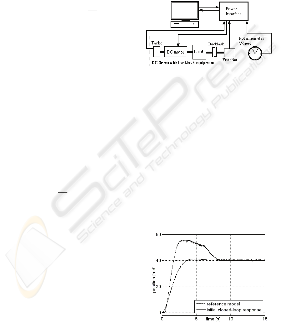
4 CASE STUDY
The experimental setup is built around the INTECO
DC servo system with backlash laboratory
equipment, Figure 5, with rated amplitude of 24 V,
current of 3.1 A, torque of 15 N cm and speed of
3000 rpm. The inertial load weighs 2.03 kg.
Figure 5: Structure of experimental setup.
The transfer functions of the simplified
controlled process and reference model are
15.1
1
)( ,
)1(
)(
2
++
=
+
=
Σ
ss
sF
sTs
k
sP
P
,
(23)
88.139
=
P
k
,
s 9198.0
=
Σ
T
. The continuous-time PI
controller has been obtained by frequency domain
design which yields the parameters
01036.0=
C
k
and
s 1043.3
=
i
T
. Discretizing with
s 01.0=
s
T
, the
initial digital PI controller parameters are
T
P
K ]0029.001035.0[
0
=α==ρ
. The parameters
obtained after 10 iterations for the step size
6
10
−
=γ
i
are
T
]003226.0010346.0[
10
=ρ
. Setting
20
=
e
B
and
5.0
=
η
, (14) results in
06452.0=
Δe
B
.
The constant reference input
rad 40=r
has been
applied. The behaviour of the CS with linear
controller before IFT is illustrated in Figure 6.
Figure 6: Reference model output and controlled output
(position) versus time for linear CS before IFT.
IFT-BASED PI-FUZZY CONTROLLERS - Signal Processing and Implementation
211

The behaviour of the CS with PI-FC after IFT is
presented in Figure 7. The performance indices
(overshoot and settling time) of the CS have been
improved. A band-limited white noise of variance
0.01 has been applied as the disturbance input d.
Figure 7: y versus time for fuzzy CS after IFT.
5 CONCLUSIONS
The paper has proposed a stable design method
dedicated to a class of Takagi-Sugeno PI-FCs. It is
based on mapping the IFT-based linear case results
onto the fuzzy control results.
Several signal processing aspects regarding the
simplification of the implementation have been
discussed. They involve an original gradient
experiment. A single gradient experiment is needed.
However an additional one can be employed in other
CS structures.
The stability analysis can be applied to the fuzzy
control of time-varying systems. It is valid because
of the quasi-continuous digital implementation of
the controllers that enables the controller design.
One future research topic concerns the
convergence analysis. Although the stability analysis
suggested is attractive, the convergence is not
guaranteed. The future research will be dedicated to
the application of the approaches to other fuzzy
controller structures (Valente de Oliveira and
Gomide, 2001; Vaščák, 2007; Pedrycz, 2009).
ACKNOWLEDGEMENTS
The paper was supported by the CNMP & CNCSIS
of Romania. The second and sixth authors are
doctoral students with the PUT. The second author is
an SOP HRD stipendiary co-financed by the
European Social Fund through the project ID 6998.
REFERENCES
Blažič, S., Škrjanc, I., 2007. Design and stability analysis
of fuzzy model-based predictive control - a case study.
J. of Intelligent and Robotic Systems. 49, 279-292.
Galichet, S., Foulloy, L., 1995. Fuzzy controllers:
synthesis and equivalences. IEEE Transactions on
Fuzzy Systems. 3, 140-148.
Hildebrand, R., Lecchini, A., Solari, G., Gevers, M., 2005.
Optimal prefiltering in Iterative Feedback Tuning.
IEEE Trans. Autom. Control. 50, 1196-1200.
Hjalmarsson, H., Gevers, M., Gunnarsson, S., Lequin, O.,
1998. Iterative Feedback Tuning: theory and
applications. IEEE Control Syst. Magazine. 18, 26-41.
Jantzen, J., 2007. Foundations of Fuzzy Control.
Chichester: Wiley.
Johanyák, Z. C., Kovács, S., 2007. Sparse fuzzy system
generation by rule base extension. In Proc. 11
th
International Conference on Intelligent Engineering
Systems (INES 2007). Budapest, Hungary, 99-104.
Kovačić, Z., Bogdan, S., 2006. Fuzzy Controller Design:
Theory and Applications. Boca Raton, FL: CRC Press.
Lam, H. K., Leung, F. H. F., 2008. Stability analysis of
discrete-time fuzzy-model-based control systems with
time delay: time-delay independent approach. Fuzzy
Sets and Systems. 159, 990-1000.
Lam, H. K., Ling, B. W. K., 2008. Sampled-data fuzzy
controller for continuous nonlinear systems. IET
Control Theory & Applications. 2, 32-39.
Michels, K., Klawonn, F., Kruse, R., Nürnberger, A.,
2006. Fuzzy Control: Fundamentals, Stability and
Design of Fuzzy Controllers. Berlin, Heidelberg, New
York: Springer Verlag.
Pedrycz, W., 2009. From fuzzy sets to shadowed sets:
interpretation and computing. International Journal of
Intelligent Systems. 24, 48-61.
Precup, R.-E., Preitl, S., Rudas, I. J., Tomescu, M. L., Tar,
J. K., 2008. Design and experiments for a class of
fuzzy controlled servo systems. IEEE/ASME
Transactions on Mechatronics. 13, 22-35.
Sala, A., Guerra, T. M., Babuška, R., 2005. Perspectives
of fuzzy systems and control. Fuzzy Sets and Systems.
156, 432-444.
Slotine, J.-J., Li, W., 1991. Applied Nonlinear Control.
Englewood Cliffs, NJ: Prentice-Hall.
Tian, E., Peng, C., 2006. Delay-dependent stability
analysis and synthesis of uncertain T-S fuzzy systems
with time-varying delay. Fuzzy Sets and Systems. 157,
544-559.
Valente de Oliveira, J., Gomide, F. A. C., 2001. Formal
methods for fuzzy modeling and control. Fuzzy Sets
and Systems. 121, 1-2.
Vaščák, J, 2007. Navigation of mobile robots using
potential fields and computational intelligence means.
Acta Polytechnica Hungarica. 4, 63-74.
Wang, W.-J., Chen, Y.-J., Sun, C.-H., 2007. Relaxed
stabilization criteria for discrete-time T-S fuzzy
control systems based on a switching fuzzy model and
piecewise Lyapunov function. IEEE Trans. Systems,
Man, and Cyber., Part B: Cybernetics. 37, 551-559.
ICINCO 2009 - 6th International Conference on Informatics in Control, Automation and Robotics
212