Layered Queuing Networks for Simulating Enterprise

Resource Planning Systems

Stephan Gradl, André Bögelsack, Holger Wittges and Helmut Krcmar

Technische Universitaet Muenchen

Abstract. As Enterprise Resource Planning systems (ERP) form the backbone

of today’s business processes the stability and performance of those systems is

vital to the whole company. In many cases less is known what happens to the

performance of an ERP system when a patch is applied or changes are made to

the ERP system. This paper presents an approach how to simulate Enterprise

Resource Planning systems (ERP) before changes are made to the system. The

approach involves the development of so called Layered Queuing Networks

(LQN). To construct such a LQN the paper utilizes a trace in the ERP system to

gather data about the internal ERP system’s architecture. These data is used to

construct a section of the internal architecture of the ERP system. The ERP sys-

tem’s architecture is transformed into a LQN and the LQN is simulated.

1 Introduction

Enterprise resource planning systems (ERP) build the backbone of today’s core busi-

ness processes. They are vital for a company’s success and are needed 24 hours a day.

But very often such complex software systems are changed without knowing the

effects of applied changes, e.g. by configuration changes. To avoid any situations of

reduced operations a kind of mechanism is needed to discover possible problems,

change results or side effects before applying any changes to the ERP system. This

can be done by simulating an ERP system. When talking about simulating ERP sys-

tems a lot of research has been done to simulate business process inside the ERP

system but not the ERP system itself [1].

An approach of simulating ERP systems is presented in [2]. The approach only of-

fers an idea of how to transfer the structure of an ERP system to a real-world struc-

ture, which may be simulated, but it lacks a recommendation about a suitable struc-

ture. This paper adopts the approach but couples with the idea of so called layered

queuing networks (LQN) [3,4]. Layered queuing networks (LQN) are an extension to

queuing networks that support the modeling of complex software systems by a com-

ponent based structure [4]. This paper utilizes the LQN approach and shows a process

how to begin a simulation process by using an exemplary ERP process and gather

data for building up the LQN. Therefore a real life business process is performed in

the ERP system and the necessary data for building up the LQN are gathered from

traces of the ERP system. The trace is ‘translated’ into a LQN and the LQN is simu-

lated using third party simulation software. The main research question for this paper

Gradl S., Böegelsack A., Wittges H. and Krcmar H. (2009).

Layered Queuing Networks for Simulating Enterprise Resource Planning Systems.

In Proceedings of the 7th International Workshop on Modelling, Simulation, Veriﬁcation and Validation of Enterprise Information Systems, pages 85-92

DOI: 10.5220/0002194200850092

 SciTePress

covers the aspect if such LQN is suitable for simulating an ERP system or not. There-

fore the developed LQN is used for simulation.

The rest of the paper is organized as follows: section 2 describes the process of

developing the LQN, which actually includes describing the exemplary business

process, analyzing the traces and creating a LQN. In section 3 the simulation of the

developed LQN is discussed. Section 4 presents related work which links to this field

of application. In section 5 the paper is summed up and presents an outlook on further

research.

2 Mapping LQN to an Exemplary ERP System

Creating a comprehensive LQN with all available components and all available data

consumes a lot of time and results in a quite huge LQN. Hence, in a first step this

paper starts with a smaller LQN containing only a limited amount of data and compo-

nents. To develop such a LQN an exemplary ERP process is chosen. To get a repre-

sentative amount of data, this process has to be a typical process the user faces in an

ERP system very often. After this process is defined on a high abstraction level the

process has to be “replayed” in the ERP system. The idea of replaying the process in

the ERP system is to gain the necessary information from a trace. The trace logs all

activities of the ERP system including the needed time for each activity. By analyzing

the trace all ERP system’s components can be detected. These components will be

used as tasks in the LQN. Moreover queuing data are provided by the trace as it

records the time which is needed to complete a request. The following figure provides

an overview about the process.

Define exemplary

ERP process

Determine ERP

system’s

components

Define LQN Simulate LQN Verify

Fig. 1. Process overview.

For realizing this process an instance of an ERP system is needed. This paper uses

a SAP® system as SAP® is the market leader in the area of ERP software. The next

chapter describes the exemplary ERP process which is used to gain the necessary

information to build up the LQN.

To draw an overview about the architecture of the SAP® system we decided to in-

troduce a typical process a user faces in the SAP® system. This is the process of

creating a material master record (MMR). A MMR can be understood as the data

structure, which represents a material in the SAP® system. It contains several data

about the material. The process for creating a MMR can be described very briefly:

1. First step is logging into the SAP® system

2. The user calls program, called transaction, for creating a MMR. The SAP® sys-

tem loads a compiled program and executes it.

3. Now the user can make some entries like material name, plant, pricing informa-

tion and others to the corresponding input fields.

4. After all necessary data is filled in the user can save the MMR. Before saving the

new MMR the SAP® system proofs validity of the values and prompts an error if

any of this validity checks fails.

5. As soon as the inputs are correct the data will be saved in the database and a con-

firmation screen will be loaded.

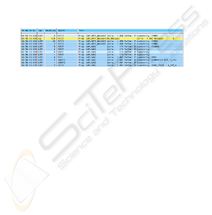
Now an internal trace is used to determine all components in the SAP® system.

The SAP® system provides the feature to trace all activities in the system for authori-

zation checks, kernel functions, kernel activities, database accesses, table buffer ac-

cesses, remote function calls, and lock activities. Tracing our exemplary ERP process

in the SAP® system provides us with the deep understanding what happens in the

SAP® system at which time. Besides the understanding the trace also provides us

with needed times for each activity.

Fig. 2. Trace showing start of the ERP process (Source: SAP®).

Figure 2 shows the first lines of a trace which was recorded when starting the ex-

emplary ERP process. The next step in the modeling and simulation process is to

determine the ERP system’s components from such a trace. This task is done manual-

ly as there is no automatic analysis software available yet. Of course, knowledge of

the theoretical architecture or an SAP® ERP System is necessary to analyze such

traces.

ERP System’s Components

To provide an understanding of the ERP system’s architecture we derive the system‘s

components from the ERP process step-by-step by analyzing the recorded trace and

the abstraction of the trace entries. These components are described in detail in [5].

1. Logging into the ERP system is done by using a front-end, so called SAPGui®.

2. The process step of calling a program involves the dispatcher process, which

assigns the user request to a disp+work process that loads a compiled version of

the program code from the database and executes it.

3. The user can change, add, and delete data now.

4. After the user has completed all necessary data and decides to save the data, the

SAPGui® sends those data to the disp+work process that performs a validity

check and prompts an error if some of the data is not correct. The user can correct

the data and try to save again.

5. As soon as the input is correct, the data is saved to the database. This is done by

the disp+work process in conjunction with a process called update process. The

process receives the data from the SAPGui® and stores the data in the corres-

ponding database tables.

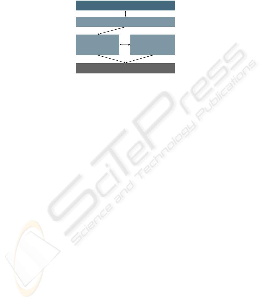
Database

SAPGui

Disp+work process

Dispatcher process

Update process

Fig. 3. Simplified SAP® system’s architecture.

Develop LQN

In Figure 3 the simplified architecture of the SAP® system is drawn. This model is

the starting point for the development of the LQN shown in Figure 4. At first the

components SAPGui®, dispatcher, disp+work process, update process, and the data-

base are modeled as tasks in the LQN. The first component is the SAPGui®, which

posts request to the system, e.g. calling a transaction. But the SAPGui® includes also

a so called think time which is “the time between successive commands” [6]. We set

the time to 3sec. The next component is the dispatcher process, which has a service

time of 484ms. The dispatcher process is called one time as the SAPGui® calls the

transaction MM01. The dispatcher forwards the request to one of the disp+work

processes. Next component is the disp+work process. We recognize that the

disp+work process must be differenced to two types of entries. The first entry (la-

beled “Normal”) describes the activities of the disp+work process during the execu-

tion of MM01 with an average execution time of 20ms. The other entry is a pre-

update activity (labeled “Pre-Update”) with an average execution time of 157ms. This

activity includes preparing the data for the update process. In the trace we recognized

that there are big time differences between both activities: 20ms and 157ms. This is

why we distinguish between normal and pre-update entry. Normal entry is called four

times during the program execution whereas the pre-update entry is called only one

time. The update process is called one time during program execution after the user

presses the save button. The disp+work process prepares the data set and activates the

update process. The trace shows an average service time 114,67ms. The database is

the most interesting part of the LQN. The LQN distinguishes between three entries:

normal, pre-update and update. The reason for this is a huge difference between the

service times. The trace shows an average service time of 4,9ms for the normal activi-

ties, e.g. loading compiled program. The pre-update activities are most time consum-

ing. The trace shows an average service time of 100ms. For the final update activity

the trace shows an average service time of 87ms. The following table 1 gives an idea

about the more detailed average service times:

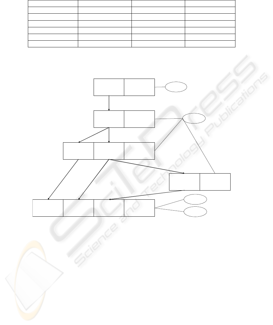
Table 1. Detailed service times.

Action Normal Pre-Update Update

Direct Read 0,33ms 0,33ms 1ms

Sequential Read 3,16ms 69,33ms 11,67ms

Update 1,25ms 0ms 1ms

Delete 0,08ms 0ms 4ms

Insert 0ms 28ms 69,67ms

Commit 0,16ms 2ms 0ms

Please note that program execution was performed two times as a warm-up phase

so that internal program buffers are filled. After warm-up phase the test was run ten

times and the LQN includes the average of these ten test run results.

SAPGuiInteract

[Z=3 s]

UserCPU

DispatcherNormal

[s=484 ms]

Disp+workPre-Update

[s=157 ms]

Normal

[s=20 ms]

DatabasePre-Update

[s=100 ms]

Normal

[s=4,9 ms]

UpdateNormal

[s=114,67 ms]

Update

[s=87 ms]

ServerCPU

Disc

ServerCPU

Fig. 4. LQN for exemplary business process.

Using the gathered data from the trace an entire LQN is built up for the exemplary

business process. This model can be used now to simulate the exemplary business

process by using simulation software and verify the LQN.

Limitations

A problem when simulating complex software systems is the decision how many

components should be simulated. Even in this little example the paper demonstrates

that a lot of data is gathered from several components in the SAP® system and that

even the database can be described in a more detailed way. In [1] an eight level archi-

tecture was presented to limit the effort of building the architecture of the SAP®

system. By analyzing the SAP® system and the traces in this work it was discovered

that the lowest level is the response time level of the database. Therefore we assume

that this can be understood as a kind of “natural edge”. As the SAP® system does not

provide more detailed information about the database the approach is to cut the simu-

lation model at this level and regard the database as a black box. Service time values

of the database are derived directly from the SAP® system. Our LQN does not con-

sider any buffers, shared memory objects etc. By analyzing the gathered trace such

information can be discovered too. As this paper present as first approach to over-

come the problems when simulating complex ERP systems, the paper focuses on a

more simple way and does not take buffers etc. into account.

3 Simulation and Verifying LQN

Simulation of layered queuing networks can be performed by a tool called LNQS.

This tool has been developed at Carleton University upon the research of the Real-

Time and Distributed Systems Group of Prof. C.M. Woodside [7]. For solving LQN

model two files are required. First, the input for the solver is the model which is

saved in an XML file. Second, a parameter file specifies several values for the simu-

lation run. Every entity (processor, task, entry, activity, every t form s of request) in

the model has to have a unique name. The entities that are referred by the different

forms of activities have to be valid. Also each entry is allowed to have only one activ-

ity bound to it.

The elements have to be parameterized. This is done in the second input file. To

specify the convergence value and the maximum number of iterations the first section

of the second input file can be used. Each task in the model has a processor. These

processors are defined in a single section. To determine the way a unit processes

requests, a scheduling strategy and the number of available instances can be assigned

to each processor. The configurations of the entries consist of their service times or

arrival rates and a definition of all calls to other entries. The output of a simulation

run contains lots of information about the behavior of the elements. This work focus-

es on the service time of the user requests as this is the performance criteria every

user perceives.

Due to our introduced LQN model and the measured service times of the aggre-

gated tasks the ERP process is simulated with 16 copies of the disp+work service and

a variable number of processors. The focus lies on the throughput of the system. Fig-

ure 5 shows the throughput in relation to the number of processors. The throughput

can be interpreted as a kind of theoretical metric for the performance of the entire

system. The maximum throughput is reached with three processors. One may expect

to see more throughput with more CPU but this has been falsified by the simulation

results.

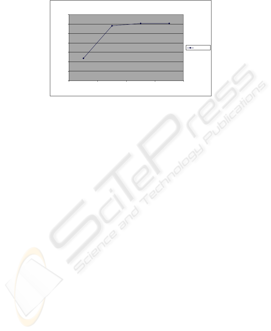
Throughput

0,820

0,840

0,860

0,880

0,900

0,920

0,940

0,960

1234

Number of CI Pr ocessors

Throughp

Throughput

Fig. 5. Normalized throughput in relation to the number of cpus.

In this scenario only a single ERP process was simulated. Simulation of parallel

ERP processes with concurrent users is not in the scope of this work.

4 Related Work

Due to their robustness and flexibility LQN Models are used for the performance

prediction of a great variety of objects. Much work is done in the area of creating

LQN models from existing models of different types. In the area of service orientated

architecture system performance characteristics [8] introduces a transformation

framework that creates LQN models of composite services out of an UML Activity

Diagram which is derived in the step before from a BPEL description of composite

service. In the area of component based software engineering there is another trans-

formation framework which creates LQNs out of a Palladio Component Model [9] to

predict response time, throughput and further important performance characteristics.

[10] presents the “component-based modelling language” which is an extension of

LQN to support the performance modelling of software consisting of sub-models of

components that are used several times. A challenge when using LQN is the problem

to get enough accurate data to build the model. To solve this problem [11] uses the

BMM method for obtaining the necessary data to predict the performance of legacy

information system. We overcome this problem by using detailed traces. Usage of

SAP® traces is also mentioned in the work of [12]. Here the traces are utilized for

giving recommendation for the automatic customizing of a SAP® system.

5 Conclusions

This paper proposes an approach towards simulating ERP systems using Layered

Queuing Networks. Therefore, an exemplary ERP business process is traced inside

the ERP system. This trace is used to determine the ERP system’s components and to

build the LQN. The LQN is simulated by using a LQN solver and simulation results

show results, which are important for real life situations, too. The paper shows, that

adding more CPU’s to a system increases the overall throughput at first but saturates

the throughput later. Instead of measuring such behavior in real life situations the

LQN approach may be used to gain information about similar situations by utilizing

simulation. Further research will focus on the behavior of LQN when dealing with a

more detailed ERP system’s architecture as well as parallel business processes and

concurrent users.

References

1. Herrmann, F., SIM-R/3: Softwaresystem zur Simulation der Regelung

produktionslogistischer Prozesse durch das R/3-System der SAP AG. In:

Wirtschaftsinformatik, Volume 49, Number 2, pp. 127-133 (2007)

2. Bögelsack, A., Jehle, H., Wittges, H., Schmidl, J., Krcmar, H., An Approach to simulate

Enterprise Resource Planning Systems. In: Proc. of the 6

International Workshop on

Modeling, Simulation, Verfificaton and Validation of Enterprise Information Systems

(MSVVEIS 2008), Barcelona, Spain. pp. 160 – 169 (2008)

3. Woodside, M., Tutorial Introduction to Layered Modeling of Software Performance, Edi-

tion 3.0, May 2002 (Accessible from http://www.sce.carleton.ca/rads/lqn/lqn-

documentation/tutorialg.pdf) (2002)

4. Ufimtsev, A., Murphy, L., Performance Modeling of a JavaEE Component Application

using Layered Queuing Networks: Revised Approach and a Case Study. 5th International

Workshop on Specification and Verification of Component-Based Systems (SAVCBS)

(2006)

5. SAP Help (Available under http://help.sap.com/erp2005_ehp_04/helpdata/DE/84/

54953fc405330ee10000000a114084/frameset.htm)

6. Jain, R., The art of computer systems performance analysis: techniques for experimental

design, measurement, simulation, and modelling. John Wiley & sons, Inc., Littleton, Mas-

sachusetts (1991)

7. Real-Time and Distributed Systems Group, Carleton University, Ottawa, Canada.

(http://www.sce.carleton.ca/rads/index.html).

8. D’Ambrogio, A., Bocciarelli, P., A Model-driven Apporach to Describe and Predict the

Performance of Composite Services. WOSP’07, Buenos Aires, Argentinia (2007)

9. Koziolek, H., Reussner, R., A Model Transformation from the Palladio Component Model

to Layered Queueing Networks. SIPEW 2008, Darmstadt, Germany (2008)

10. Wu, X., Woodside, M., Performance Modeling from Software Components. Workshop on

Simulation and Performance (2004)

11. Jin, Y., Tang, A., Han, J., Liu, Y., Performance Evaluation and Prediction for Legacy

Information Systems. 29th International Conference on Software Engineering (2007)

12. Rene Schult, Gamal Kassem: SELF-ADAPTIVE CUSTOMIZING WITH DATA MINING

METHODS - A Concept for the Automatic Customizing of an ERP System with Data Min-

ing Methods. In Proceedings of ICEIS 2008 (2008)

13. Svobodovva, L., Computer Performance Measurement and Evaluation Methods: Analysis

and Applications. American Elsevier Publishing Company, Inc., New York (1976)