ON THE STATE–SPACE REALIZATION OF VECTOR

AUTOREGRESSIVE STRUCTURES

An Assessment

Vasilis K. Dertimanis, Dimitris V. Koulocheris

Vehicles Laboratory, National Technical University of Athens, Iroon Politechniou 9, 157 80, Athens, Greece

Keywords:

Vector autoregressive, Time–series, State–space, Green function, Covariance matrix, Dispersion analysis, Es-

timation.

Abstract:

This study explores the interconnection between vector autoregressive (VAR) structures and state–space mod-

els and results in a compact framework for the representation of multivariate time–series, as well as the esti-

mation of structural information. The corresponding methodology that is developed, applies the fact that every

VAR process of order n may be described by an equivalent (non–unique) VAR model of ﬁrst order, which is

identical to a state–space realization. The latter uncovers many ”hidden” information of the initial model, it

is more easy to manipulate and maintains signiﬁcant second moments’ information that can be reﬂected back

to the original structure with no effort. The performance of the proposed framework is validated using vector

time–series signatures from a structural system with two degrees of freedom, which retains a pair of closely

spaced vibration modes and has been reported in the relevant literature.

1 INTRODUCTION

The analysis of vector time–series, generally referring

to the determination of the dynamics that govern the

performance of a system under unobservable excita-

tions, has been a subject of constant development for

more than two decades, as part of the broader system

identiﬁcation framework. Relative applications are

extended from econometrics (Clements and Henry,

1998; L¨utkepohl, 2005), to dynamics (Ljung, 1999;

Koulocheris et al., 2008), vibration (Papakos and Fas-

sois, 2003), modal analysis (Huang, 2001) and fault

diagnosis (Dertimanis, 2006).

The study of vector time–series can be assessed

from a variety of viewpoints, with respect to the ap-

plication of interest. These include simulation, pre-

diction and extraction of structural information. Yet,

while in the ﬁrst two areas the interrelation of the cor-

responding time–series structures, such as the VAR

one (or the VARX and the VARMAX, under the

availability of input information), to equivalent state–

space models has been studied extensively (Hannan,

1976; Brockwell and Davis, 2002; L¨utkepohl, 2005),

not much have been done in the third (Lardies, 2008),

from where it appears that state–space realizations

may provide signiﬁcant advantages, regarding struc-

tural estimation, with respect to other approaches (He

and Fu, 2001).

This paper attempts to provide a uniﬁed frame-

work for the representation of vector time–series, by

means of VAR structures and their corresponding

state–space realizations. Based on the fact that ev-

ery VAR structure of order n (referred to from now on

as VAR(n) structure) can be expressed as an equiva-

lent (and non–unique) VAR(1) one, a corresponding

state–space model is developed. This speciﬁc model

qualiﬁes, over other possible realizations, for having

a transition matrix that coincides with the VAR(n)

polynomial matrix. It turns out that the spectrum of

this transition matrix has all the structural information

about the system that generates the time–series ”hid-

den” in its spectrum. Consequently, by taking advan-

tage standard results of matrix algebra, closed form

expressions for the Green function and the covariance

matrix are derived. The latter, unlike other estimation

schemes, such as the Burg and the forward–backward

methods (Brockwell and Davis, 2002), is by deﬁnition

closely related to the energy distribution of the vec-

tor time–series. Thus, the corresponding expression

that is assessed, quantiﬁes the impact of each speciﬁc

structural mode in the total energy of the system, a

technique that has been recorded in the literature as

K. Dertimanis V. and V. Koulocheris D. (2009).

ON THE STATE–SPACE REALIZATION OF VECTOR AUTOREGRESSIVE STRUCTURES: AN ASSESSMENT.

In Proceedings of the 6th International Conference on Informatics in Control, Automation and Robotics - Signal Processing, Systems Modeling and

Control, pages 20-27

DOI: 10.5220/0002188100200027

 SciTePress

dispersion analysis (Lee and Fassois, 1993).

The paper is organized as follows: in Sec. 2 the

VAR(n) structure is presented and the reduction to the

state–space realization is performed. Section 3 illus-

trates the properties of the state–space model, includ-

ing the development of closed form representations

for the Green function and the covariance matrix, and

how these are reﬂected to the original VAR(n) struc-

ture. Section 4 contains the least–squares estimation

of the state equation and Sec. 5 the validation of the

estimated model, as well as the extraction of the struc-

tural information that is ”hidden” in the transition ma-

trix. Section 6 displays an application of the proposed

framework to a simulated vibrating system that has

been already used in the past (Lee and Fassois, 1993;

Fassois and Lee, 1993) and in Sec. 7 the method is

concluded and some remarks for further research are

outlined.

2 THE VAR(n) STRUCTURE

2.1 The Model

Let Y[t] =

[t] y

[t] ... y

[t]

denote a s–

dimensional vector time–series of zero mean random

variables

. Under the stationarity assumption (Box

et al., 2008), Y[t] can be described by a ﬁnite order

VAR model of the following form:

Y[t] + A

·Y[t −1] + ... + A

·Y[t −n] = Z[t] (1)

In the above equation n is the order of the VAR pro-

cess, A

designate the [s×s] AR matrices and Z[t] de-

scribes a vector white noise process with zero mean,

≡ E

Z[t]

= 0 (2)

and covariance function,

[h] ≡ E

Z[t + h]·Z

[t]

(

h = 0

0 h 6= 0

(3)

where Σ

Σ is a non–singular (and generally non–

diagonal) matrix.

Taking advantage of the backshift operator q, de-

ﬁned such that q

−k

·Y[t] = Y[t −k], the VAR(n) struc-

ture can be compactly written as,

A(q)·Y[t] = Z[t] (4)

where A(q) is the [s×s] AR polynomial matrix:

A(q) = I

+ A

·q

−1

+ ... + A

·q

−n

(5)

Throughout the paper, quantities in the brackets shall

notate discrete–time units (or time lags, in the case of co-

variance functions) and hats shall notate estimators / esti-

mates. E{·} shall notate expectation.

2.2 Reduction to State–space

Any VAR(n) process of Eq. 1 can be transformed to an

equivalent VAR(1) structure (L¨utkepohl, 2005). De-

ﬁne the [n·s×1] vectors,

Ξ[t] =







Y[t −n + 1]

Y[t −n + 2]

Y[t −1]

Y[t]







N[t] =







Z[t]







(6)

and the [n·s×n·s] and [s×n·s] matrices,

F =







... O

... ...

... I

−A

n−1

... −A







(7)

C =



... I



(8)

respectively, Eq. 1 can take the following form:

Ξ[t] = F·Ξ

Ξ[t −1] + N

N[t] (9)

Y[t] = C·Ξ

Ξ[t] (10)

Equations 9–10 illustrate the state–space realization

of the VAR(n) structure of Eq. 1. Naturally, the state–

space model consists of a state equation (Eq. 9), in

which F is the state transition matrix, and an obser-

vation equation (Eq. 10) that relates the original s–

variate time–series Y[t] to the state vector, Ξ

Ξ[t], by

means of the output matrix C. Obviously, the state

equation can be viewed as a VAR(1) model, in which

Ξ[t] is a well–deﬁned stationary stochastic process

and N[t] has properties similar to that of Z[t], as it

will become clear at the following.

It must be noted that the state–space realization

of Eq. 1 is not unique (Lardies, 2008). In fact they

exist inﬁnitely many pairs {F,C} that can describe

Y[t] in terms of Eqs. 9–10, since any transformation

of the state vector by a non–singular [n·s ×n·s] ma-

trix T leads to new state equation, in which the transi-

tion matrix T·F·T

−1

is similar to F and preserves its

eigenvalues (Meyer, 2000). Yet, Eq. 1 has a very im-

portant property: the transition matrix F, as deﬁned

in Eq. 7, is the block companion matrix of the poly-

nomial matrix A(q) described by Eq. 5 and includes

all the structural information of interest, regarding the

process that generates the s–variate time–series Y[t].

ON THE STATE-SPACE REALIZATION OF VECTOR AUTOREGRESSIVE STRUCTURES: AN ASSESSMENT

3 PROPERTIES OF THE

STATE–SPACE REALIZATION

3.1 Noise

From Eqs. 6, 8, it holds that,

N[t] = C

·Z[t] (11)

so the mean value and the covariance matrix of N[t]

are given by,

≡ E

N[t]

= C

·E

Z[t]

= 0 (12)

and,

[h] ≡ E

N[t + h]·N

[t]

= E

·Z[t + h]·Z

[t]·C

= C

·E

Z[t + h]·Z

[t]

·C

= C

·Γ

[h]·C (13)

leading to,

[h] =

(

h = 0

0 h 6= 0

(14)

where Σ

= C

·Σ

·C.

3.2 State Vector

Since the state transition equation reﬂects the prop-

erties of an observed dynamic system, the output of

which is the available s–variate time–series Y[t], it

is desirable to obtain corresponding mathematical ex-

pressions that assess and quantify the relative infor-

mation. Conventional time–series analysis usually is

led to inﬁnite, or recursive expressions for the repre-

sentation / calculation of valuable quantities, such as

the weighting function (referred to also as Greenfunc-

tion, process generating function, or transfer func-

tion) and the covariance matrix. The analysis that

follows leads to closed form representations, which

reveal the spectral characteristics of the transition ma-

trix F.

3.2.1 The Green Function

Starting from the VAR(1) state equation,

Ξ[t] = F·Ξ

Ξ[t −1] + N

N[t] (15)

it can be written as an inﬁnite vector moving average,

Ξ[t] =

∞

∑

k=0

·N

N[t −k] (16)

which is a multivariate generalization of Wold’s the-

orem (Box et al., 2008). Without loss of generality,

assuming that F has a complete set of eigenvalues



,λ

,...,λ

n·s



, it can be expressed as,

F =

n·s

∑

j=1

·λ

(17)

where G

are the spectral projectors of F (refer to

the Appendix for a brief introduction to the spectral

properties of square matrices). The substitution of

Eq. 17 to Eq. 16, using the fact that G

= G

and

·G

= 0, i 6= j, yields,

Ξ[t] =

∞

∑

k=0

n·s

∑

j=1

·λ

·N

N[t −k]

∞

∑

k=0

n·s

∑

j=1

·λ

·N

N[t −k]

∞

∑

k=0

[k]·N

N[t −k] (18)

so that the coefﬁcients of the weighting (Green) func-

tion can be expressed in a closed form as,

[k] ≡ F

n·s

∑

j=1

·λ

(19)

in terms of the spectrum of F. Notice that by deﬁ-

nition (Eq. 16), H

[k] can be viewed as the impulse

response of the state difference equation, which gen-

erally has a decaying performance, characterized by

a mixture of damped exponentials and cosines, as for

example in vibrating systems, where the eigenvalues

often appear in complex conjugate pairs. Further-

more it holds that (see Appendix):

[0] =

n·s

∑

j=1

= I (20)

3.2.2 The Covariance Matrix

The covariance matrix related to the Wold decompo-

sition of the state equation is (Brockwell and Davis,

2002):

[h] =

∞

∑

k=0

k+h

·Σ





(21)

Using Eq. 17, the following apply:

ICINCO 2009 - 6th International Conference on Informatics in Control, Automation and Robotics

[h] =

∞

∑

k=0

(

n·s

∑

j=1

·λ

k+h

·Σ

n·s

∑

m=1

·λ

)

∞

∑

k=0

(

n·s

∑

j=1

·λ

k+h

·Σ

n·s

∑

m=1

·λ

)

∑

·Σ

·G

·λ

∞

∑

k=0

·λ

∑

·Σ

·G

·λ

1−λ

·λ

n·s

∑

j=1

·Σ

n·s

∑

m=1

1−λ

·λ

(22)

Setting,

= G

·Σ

n·s

∑

m=1

1−λ

·λ

(23)

the covariance matrix can be expressed as:

[h] =

n·s

∑

j=1

·λ

(24)

Equation 24 has some important features. First, as

become directly evident, it has the same form as the

Green function. Second, it describes the covariance

matrix in terms of the spectral properties of the tran-

sition matrix (plus the noise covariance), which, as

already mentioned, contains all the information about

the dynamics that produce the state vector and, thus,

Y[t]. This fact leads to a third crucial feature: for

h = 0, Eq. 24 yields:

[0] = D

+ D

+ ···+ D

n·s

(25)

Recalling that Γ

[0] can be treated as the multivari-

ate equivalent of the variance (in fact its diagonal ele-

ments are the variances of each entry of Ξ

Ξ[t]), Eq. 25

can be used as a direct measure of the signiﬁcance that

every eigenvalue has, in the total energy of the vector

time–series. This leads to the notion of dispersion

analysis, originated in the work of (Lee and Fassois,

1993), in which the estimated modal characteristics

of a vibrating system are qualiﬁed against some pre-

deﬁned thresholds. In the next section, a more practi-

cal version of Eq. 25 is presented, with respect to the

estimation problem.

In the case that the correlation matrix is of interest,

it can be calculated from (Box et al., 2008),

[h] = V

−1/2

·Γ

[h] ·V

−1/2

(26)

where V

is a diagonal matrix that contains the auto-

correlations at zero lag:

−1/2

= diag



−1/2

[0],...,γ

−1/2

n·s

[0]



(27)

3.3 Output Time–series

The previous analysis explored the advantages of the

state equation and led to closed form representations

for the coefﬁcients of the Green function and the co-

variance matrix, which are exclusively depend on the

spectrum of the transition matrix F. Naturally, there

exist strong connections between these quantities and

the corresponding ones of the s–variate time–series

Y[t]. The link is just the output equation of the state–

space model. The substitution of Eq. 16 to Eq. 10,

under the result of Eq. 19, yields,

Y[t] = C·Ξ

Ξ[t] = C·

∞

∑

k=1

·N

N[t −k]

∞

∑

k=0

C·H

[k]·C

·Z

Z[t −k]

∞

∑

k=0

[k] ·Z

Z[t −k] (28)

where:

[k] = C·H

[k]·C

n·s

∑

j=1

C·G

·C

·λ

n·s

∑

j=1

Ω

·λ

(29)

The covariance matrix of Y[t] is:

[h] ≡ E

Y[t + h]·Y

[t]

∞

∑

k=0

[k+ h] ·Σ

·H

[k] (30)

Recalling that,

= C

·Σ

·C (31)

and

[k] = C·H

[k]·C

(32)

the following apply:

[h] =

∞

∑

k=0

C·H

[k+ h]·C

·Σ

·C·H

[k]·C

= C·

(

∞

∑

k=0

[k+ h]·Σ

·H

[k]

)

·C

= C·Γ

[h] ·C

(33)

Thus, from Eq. 24,

[h] =

n·s

∑

j=1

·λ

(34)

ON THE STATE-SPACE REALIZATION OF VECTOR AUTOREGRESSIVE STRUCTURES: AN ASSESSMENT

where,

= C·D

·C

(35)

while if the correlation matrix R

[h] is needed, corre-

sponding versions of Eqs. 26– 27 apply to Eq. 34 as

well.

Equations 29 and 34 show how the properties of

the s–variate time–series Y[t] are related to the transi-

tion matrix. It is important to observe that the above

analysis is strictly depended on the spectrum of F. In-

deed, when the VAR(n) structure described by Eq. 1

is available, all the information about the dynamics

of the system that produces Y[t] can be assessed by

the eigenvalue problem of F, the state transition ma-

trix of the state–space realization, which is identical to

the block companion matrix of the polynomial matrix

A(q). Of course, no VAR structure exists a–priori for

an available data set and it rather has to be estimated.

This is the topic of the next Section.

4 ESTIMATION

The estimation of VAR(n) structures pertains to the

identiﬁcation of the polynomial matrix order and co-

efﬁcients, as well as the covariance matrix of the vec-

tor noise sequence, given observations of a s–variate

times–series Y[t], t = 1,...,N, that has been sampled

at a period T

. To this, the state–space realization may

again be utilized, noting that, regardless the selected

order n of the original VAR structure, the state equa-

tion retains the ﬁrst order VAR form. In addition,

Eq. 15 can be written as a linear regression,

Ξ[t] = Φ

Φ[t]·f

f + N[t] (36)

with,

Φ[t] = −Ξ

[t −1] ⊗I

n·s

[n·s×n·s

] (37)

f = vec





[n·s

×1] (38)

where ⊗ denotes Kronecker’s product and vec{·} the

vector that is produced by stacking the columns of the

relative matrix, one underneath the other. Introduc-

ing,

Ξ =

[1] ... Ξ

[N]

[N·n·s×1] (39)

Φ =

Φ[1] ... Φ

Φ[N]

[N·n·s×n·s

] (40)

N =

[1] ... N

[N]

[N·n·s×1] (41)

the minimization of the quadratic norm,

V( f

f) =

·N

·Λ

Λ·N (42)

where N = Ξ

Ξ −Φ

Φ·f

f and Λ

Λ any arbitrary weight-

ing matrix (the covariance of the residual vector N

is presently utilized, calculated as I

⊗

−1

), leads

to the well-known normal equations for the least–

squares estimation of f

·Φ

Φ·

f = Φ

·Ξ

Ξ (43)

whereas the covariance matrix associated with the es-

timate of Eq. 43 is:

P =



·Λ

Λ·Φ



−1

(44)

The diagonal entries of P are the variances of the pa-

rameter vector f

f. Thus, assuming normality (pro-

vided that N ≫ n·s

), the 95% conﬁdence limits are

derived from

±1.96·σ

for j = 1,... , n·s

. Note

that if the zero value is contained in this interval, the

relative parameter can be regarded as zero.

Having the state equation estimated, the transition

to the original VAR(n) structure is designated by the

matrix C of the state–space realization’s output equa-

tion. To this, the transformation methods that were

implied in Sec. 3 are applied.

5 VALIDATION

The vector time–series ﬁtting strategy consists of

ﬁnding an appropriate estimate of the order n, as

well as of exploring the properties of the innovations,

Z[t]. Both may be qualiﬁed via minimization of the

Bayesian Information Criterion (BIC), deﬁned as,

BIC = ln det |

|+ n·s

ln N

(45)

while the innovations can be further tested for white-

ness, using standard hypothesis tests. See (Papakos

and Fassois, 2003) for details.

Once the ﬁnal model has been available, com-

plete structural information can be assessed in terms

of the estimated transition matrix. Towards this, the

spectrum of

F is calculated, namely the eigenvalues

and the eigenvectors, while using Eq. 34, the relative

importance of each structural mode, within the total

energy of the system is evaluated. With respect to

the discussion that took place in Sec. 3.2.2, regarding

the notion of the dispersion analysis, setting h = 0 in

Eq. 34 yields:

[0] = Q

+ Q

+ ···+ Q

n·s

(46)

Let γ

be the [i, j] element of Γ

[0]. Then,

= q

1 ij

+ q

2 ij

+ ···+ q

n·s ij

(47)

and since the eigenvalues of the transition matrix usu-

ally come as a mixture of real and complex conjugate

ICINCO 2009 - 6th International Conference on Informatics in Control, Automation and Robotics

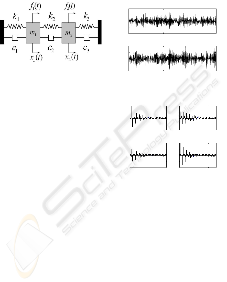
Figure 1: A structural system with two degrees of free-

dom: m

= m

= 4.5 kg, c

= 45 Ns/m, c

= 35 Ns/m,

= 15 Ns/m, k

= k

= 17500 N/m, k

= 100 N/m

numbers, the structural dispersions within the content

of the [i, j] covariance estimate are deﬁned as:

Real mode:

ij k

= q

ij k

(48)

Complex mode:

ij k

= q

ij k

+ q

∗

ij k

(49)

Thus, the relative importance of each dispersion in the

[i, j] covariance estimate is:

∆

ij k

×100% (50)

This procedure allows the determination of the contri-

bution of the k

identiﬁed mode in every element of

the covariance matrix, by building corresponding ∆

∆

which store the relative normalized dispersions ∆

ij k

6 EXPERIMENTAL VALIDATION

The method’s performance was examined through the

structural identiﬁcation problem of a vibrating system

with two degrees of freedom, presented in Fig. 1. The

system is characterized by a pair of closely spaced

modes, as indicated in Tab. and the vector time–series

used for the identiﬁcation tasks was the vibration dis-

placement of the masses. The statistical consistency

of the method was investigated via Monte Carlo anal-

ysis that consisted of 20 data records of vibration dis-

placement time–series (with each such record having

1000 samples, see Fig. 2 for a single realization and

Fig. 3 for its covariance matrix), obtained with dif-

ferent white excitations and noise–corrupted at 5%

noise to signal (N/S) ratio. Regarding the simula-

tion, the continuous system was discretized using the

impulse–invariant transformation, at a sampling pe-

riod T

= 0.025 s.

0 5 10 15 20 25

−2

−1

Time (s)

[t]

Vibration displacement time−series

0 5 10 15 20 25

−2

−1

Time (s)

[t]

Figure 2: A realization of the noise corrupted (at 5% N/S

ratio) vibration displacement time–series.

0 20 40

−1

−0.5

0.5

TS 1

lag τ

ACF

0 20 40

−1

−0.5

0.5

TS 1 x TS 2

lag τ

CCF

0 20 40

−1

−0.5

0.5

TS 2 x TS 1

lag τ

CCF

0 20 40

−1

−0.5

0.5

TS 2

lag τ

ACF

Figure 3: The correlation matrix of the series in Fig. 2 for

50 lags. TS1: x

[t], TS2: x

[t], ACF: autocorrelation, CCF:

cross–correlation.

Following the estimation procedure described in

Sec. 5, a VAR(2) structure was found adequate to de-

scribe system dynamics. Table 1 illustrates the esti-

mates of the natural frequencies and the damping ra-

tios (in fact the corresponding mean values and the

standard deviations of the Monte Carlo simulation),

together with the theoretical ones, from where it is

clear that the method performed satisfactory and iden-

tiﬁed the relative quantities, even in the absence of the

input excitations. Table 1 further displays the percent-

age dispersion matrices for each mode of vibration,

showing that the second mode is a heavier contributor

in the total energy of the system. This result coincides

with the previous assessment of the speciﬁc simulated

system, reported in (Fassois and Lee, 1993).

For further validation of the results, Figs. 4–5 dis-

play the theoretical correlationmatrix of the estimated

model for the vector time–series of Fig. 1 and the

sample correlation matrix of the innovations, for the

ON THE STATE-SPACE REALIZATION OF VECTOR AUTOREGRESSIVE STRUCTURES: AN ASSESSMENT

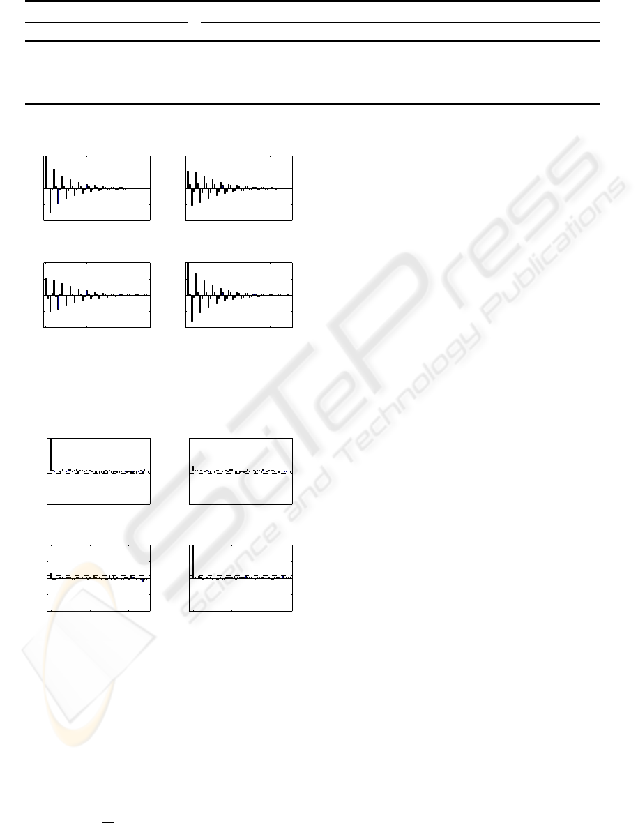
Table 1: Theoretical / identiﬁed natural frequencies (Hz) and damping ratios and dispersions of the identiﬁed VAR(n) struc-

ture.

Dispersion matrices (%)

Theoretical Identiﬁed 1

Mode

9.9793 9.9903±0.1446



37.68±5.06 −32.95±8.82

−37.01±10.18 9.58±2.73

 

62.32±5.06 132.95±8.82

137.01±10.18 90.42±2.73



9.9274 9.9307±0.0636

ζ 0.1826 0.1848±0.0174

0.0480 0.0477±0.0073

0 20 40

−1

−0.5

0.5

TS 1

lag τ

ACF

0 20 40

−1

−0.5

0.5

TS 1 x TS 2

lag τ

CCF

0 20 40

−1

−0.5

0.5

TS 2 x TS 1

lag τ

CCF

0 20 40

−1

−0.5

0.5

TS 2

lag τ

ACF

Figure 4: Theoretical correlation matrix: estimated model

for the series in Fig. 2 (50 lags). Notation is the same as in

Fig. 3.

0 20 40

−1

−0.5

0.5

TS 1

lag τ

ACF

0 20 40

−1

−0.5

0.5

TS 1 x TS 2

lag τ

CCF

0 20 40

−1

−0.5

0.5

TS 2 x TS 1

lag τ

CCF

0 20 40

−1

−0.5

0.5

TS 2

lag τ

ACF

Figure 5: Sample correlation matrix: innovations of the es-

timated model for the series in Fig. 2 (50 lags). Notation is

the same as in Fig. 3.

same model. The estimated theoretical correlation is

very accurate, it follows its sample counterpart and

exhibits a damped sinusoidal behavior, as a result of

the identiﬁed complex conjugate eigenvalues of the

transition matrix. In addition, the sample correlations

of the innovations satisfy the whiteness hypothesis

test, at a 95% level of signiﬁcance, since they are kept

within the 1.96/

√

N thresholds (Fig. 5, dash lines).

7 CONCLUSIONS

A novel method for the representation of vector time–

series, by means of VAR(n) structures, was presented

in this paper. Focusing on the estimation of struc-

tural information, the method takes advantage of the

fact that every VAR(n) structure can be turn into a

VAR(1) counterpartand is led to a state–space realiza-

tion, whose transition matrix coincides with the block

companion matrix of the VAR polynomial. Conse-

quently, it is shown how important quantities of the

original VAR(n) structure, such as the Green function

and the covariance matrix, can be qualiﬁed and as-

sessed only in terms of the spectrum of the transition

matrix. This fact provides the user with the ability

to accurately evaluate the signiﬁcance of every struc-

tural mode in the total vector time–series energy (a

technique referred to as dispersion analysis). Of the

advantages of the method is the avoidance of itera-

tive iteration schemes and the estimation of a unique

structure for a given data set.

The encouraging results (reduced data acquisition,

statistical consistency, accurate structural identiﬁca-

tion, no overdetermination, unique estimate) suggest

the further research into this ﬁeld. Extension of the

method to vector time–series with structural indices

governed by multiple eigenvalues, probably by means

of Jordan canonical forms, as well as the investiga-

tion of VARMA models, ensues straightly. Of main

interest is also the application of the method under

the availability of input excitation and the expansion

of its framework to non–stationaryvector time–series,

to closed–loop operations, as well as to fault diagno-

sis schemes.

REFERENCES

Box, G., Jenkins, G., and Reinsel, G. (2008). Time Series

Analysis, Forecasting and Control. Prentice–Hall In-

ternational, New Jersey, 4

edition.

Brockwell, P. and Davis, R. (2002). Introduction to Time

Series and Forecasting. Springer–Verlag, New York.

ICINCO 2009 - 6th International Conference on Informatics in Control, Automation and Robotics

Clements, M. and Henry, D. (1998). Forecasting Economic

Time Series. Cambridge University Press, Cam-

bridge.

Dertimanis, V. (2006). Fault Modeling and Identiﬁcation

in Mechanical Systems. PhD thesis, School of Me-

chanical Engineering, GR 157 80 Zografou, Athens,

Greece. In greek.

Fassois, S. and Lee, J. (1993). On the problem of stochas-

tic experimental modal analysis based on multiple–

excitation multiple–response data, Part II: The modal

analysis approach. Journal of Sound and Vibration,

161(1):57–87.

Hannan, E. (1976). The identiﬁcation and parameterization

of ARMAX and state space forms. Econometrica,

44(4):713–723.

He, J. and Fu, Z.-F. (2001). Modal Analysis. Butterworth–

Heinemann, Oxford.

Huang, C. (2001). Structural identiﬁcation from ambient

vibration using the multivariate AR model. Journal

of Sound and Vibration, 241(3):337–359.

Koulocheris, D., Dertimanis, V., and Spentzas, C. (2008).

Parametric identiﬁcation of vehicle structural charac-

teristics. Forschung im Ingenieurwesen, 72(1):39–51.

Lardies, J. (2008). Relationship between state–space and

ARMAV approaches to modal parameter identiﬁca-

tion. Mechanical Systems and Signal Processing,

22(3):611–616.

Lee, J. and Fassois, S. (1993). On the problem of stochas-

tic experimental modal analysis based on multiple–

excitation multiple–response data, Part I: Dispersion

analysis of continuous–time systems. Journal of

Sound and Vibration, 161(1):57–87.

Ljung, L. (1999). System Identiﬁcation: Theory for the

User. Prentice–Hall International, New Jersey, 2

edition.

L¨utkepohl, H. (2005). New Introduction to Multiple Time

Series Analysis. Springer–Verlag, Berlin.

Meyer, C. (2000). Matrix Analysis and Applied Linear

Algebra. Society for Industrial and Applied Mathe-

matics, Philadelphia.

Papakos, V. and Fassois, S. (2003). Multichannel identiﬁca-

tion of aircraft skeleton structures under unobservable

excitations: A vector AR/ARMA framework. Me-

chanical Systems and Signal Processing, 17(6):1271–

1290.

APPENDIX: MATRIX SPECTRUM

Every [n×n] matrix A with spectrum,

σ(A) = {λ

,λ

,...,λ

}, k ≤ n (51)

has the following properties (Meyer, 2000):

- It is similar to a diagonal matrix.

- It retains a complete linearly independent set of

eigenvectors.

- Every λ

is semi–simple.

Any such matrix can be written as,

A = λ

·G

+ λ

·G

+ ... + λ

·G

(52)

where the G

’s are the, so called, spectral projectors,

for which the following properties hold:

⊲ G

+ G

+ ... + G

= I

⊲ G

·G

= 0, i 6= j

⊲ G

= G

There are various ways to calculate the spectral pro-

jectors. Among them, the one that is presently utilized

uses only the matrix A and its eigenvalues λ

to com-

pute G

∏

i=1

i6= j



A−λ

·I



∏

i=1

i6= j



−λ



(53)

ON THE STATE-SPACE REALIZATION OF VECTOR AUTOREGRESSIVE STRUCTURES: AN ASSESSMENT