A MULTI-OBJECTIVE APPROACH TO APPROXIMATE THE
STABILIZING REGION FOR LINEAR CONTROL SYSTEMS
Gustavo S
´
anchez, Miguel Strefezza
Universidad Sim
´
on Bolivar, Departamento de Procesos y Sistemas, Venezuela
Orlando Reyes
Universidad Sim
´
on Bolivar, Departamento de Tecnologia Industrial, Venezuela
Keywords:
Stabilizing Region, Controller Design, PID Control, Randomized Algorithms, Genetic Algorithms.
Abstract:
Stability is a crucial issue to consider for control system design. In this paper a new multi-objective approach
to approximate the stabilizing region for linear control systems is proposed. The design method comprises
two stages. In the first stage, a bi-objective sub-problem is solved: the algorithm aims to calculate the vertices
that maximize both the volume of the decision space and the percent of stable individuals generated within
the decision space. In the second stage, the information gathered during the first stage is used to solve the
actual multi-objective control design problem. To evaluate the proposed method a PID design problem is
considered. Results show that in this case, our method is able to find better Pareto approximations than the
classical approach.
1 INTRODUCTION
Multi-Objective Evolutionary Algorithms (MOEA)
have been succesfully applied to control applica-
tions, provided the optimization problem can not be
solved by classical methods (Fleming, 2001),(Tan
et al., 2005). However, these algorithms often oper-
ate in a fixed search space predefined a priori, which
hopefully contains the stabilizing region (Khor et al.,
2002). Note that this requirement is hard to fulfil in
practical control applications, since in general there is
little information about the geometry of the stabilizing
region. However, the stability of a control system is
extremely important and is generally a safety issue.
Evolutionary computation techniques assume the
existence of an efficient evaluation of the feasible in-
dividuals. However, there is no uniform methodo-
logy for evaluating unfeasible ones. In fact, several
techniques have been proposed to handle constraints
within the framework of MOEAs. The simplest ap-
proach is for example to reject unfeasible solutions
(Michalewicz, 1995). In this work, we propose to
determine an approximation of the stabilizing region
trying to generate and to keep feasible individuals
during the whole search process. Note that in practice
the information about the stabilizing region is very
important for the control engineer.
Quite surprisingly, there exist few references
about MOEAs which consider a dynamic search
space. As an example, a multi-population algo-
rithm called Multi-Objective Robust Control Design
(MRCD) was proposed in (Herreros, 2000). The
search space is dynamic and a filtered elite is em-
ployed to preserve the best results for future gene-
rations.
In (Arakawa et al., 1998) an algorithm called
Adaptive Range Genetic Algorithm (ARange GA)
was described. The searching range is adapted in such
a way that there is no need to define the initial range
and nor the number of bits to determine the precision
of results, if binary codification is adopted.
In (Khor et al., 2002) an inductive/deductive
learning approach for single and multi-objective evo-
lutionary optimization was proposed. The method
is able of directing evolution towards more promi-
sing search regions even if these regions are outside
the initial predefined space. For problems where the
global optimum is included in the initial search space,
it is able of shrinking the search space dynamically
for better resolution in genetic representation.
Another algorithm called ARMOGA (Adaptive
Range Multi-Objective Genetic Algorithm) was pro-
153
Sánchez G., Strefezza M. and Reyes O. (2009).
A MULTI-OBJECTIVE APPROACH TO APPROXIMATE THE STABILIZING REGION FOR LINEAR CONTROL SYSTEMS.
In Proceedings of the 6th International Conference on Informatics in Control, Automation and Robotics - Intelligent Control Systems and Optimization,
pages 153-158
DOI: 10.5220/0002181601530158
Copyright
c
 SciTePress

posed in (Sasaki et al., 2002). Based on the statistics
of designs computed so far, the new decision space
is determined. The authors claim that their algorithm
makes possible to reduce the number of evaluations to
obtain Pareto solutions.
In other hand, randomized techniques for analy-
sis of uncertain systems have attracted considerable
interest in recent years, and a significant amount of
results have appeared in the literature (Calafiore and
Dabbene, 2006). The basic idea is to characterize
uncertain parameters as random variables, and then
to evaluate the performance in terms of probabilities.
Analogously, probabilistic synthesis is aimed at deter-
mining the parameters so that certain desired levels of
performance are attained with high probability.
In the following, a new randomized multi-
objective approach to determine an approximation of
the stabilizing region for linear controllers is pre-
sented. The design method comprises two stages. In
the first stage a bi-objective sub-problem is solved:
the vertices that maximize both the volume of the de-
cision space and the ratio of feasible individuals are
calculated. In the second stage, the information gath-
ered during the first stage is used to solve the actual
multi-objective control design problem.
To evaluate the proposed method a PID design
problem is considered. Note that these controllers are
still the preferred structure in most industries. And
this is because of several reasons. From a practical
view, they come pre-programmed in most commer-
cial controllers and are well understood by both en-
gineers and technicians. Thus, it is important to ve-
rify whether any design problem can be solved using
a PID structure, before testing more complex solu-
tions.
In the framework of this paper, we have another
important motivation to consider PID controllers.
Recently, Hohenbichler et al (2008) developed a
MATLAB
R

toolbox, called PIDROBUST, which
allows to calculate the stability region of control loops
which contain an ideal PID controller. This is why
we propose to evaluate the quality of the the bound-
aries which are going to be estimated in this paper
by means of the new proposed randomized multi-
objective approach.
The paper is organized as follows. In section 2,
the design problem is formulated. In section 3 the
proposed design method is described. In section 4,
numerical results are given and finally in section 5
conclusions are given.
Figure 1: Control loop with a PID controller.
2 PROBLEM FORMULATION
Consider the control loop in figure 1. Therein, the
ideal PID controller has the equation shown in (1).
Blocks W
n
(s) and W
d
(s), s ∈ C represent arbitrary
filters. The signals r(s), d(s) and n(s) represent the
reference, disturbance and noise signals respectively.
For regulation problems it is assumed r(s) = 0 and
then equations (2), (3) and (4) hold.
K
PID
(s) =
K
D
s
2
+ K
P
s + K
I
s
(1)
y(s) = −T (s)W
n
(s)n(s) + S(s)W
d
(s)d(s) (2)
T (s) =
K
PID
(s)G(s)
1 + K
PID
(s)G(s)
(3)
S(s) =
1
1 + K
PID
(s)G(s)
(4)
The transfer functions S(s) and T (s) are known
as sensitivity function and complementary sensiti-
vity function respectively. To attenuate disturbance
and noise signals, both S(s) and T (s) must be made
“small”. However, note that from equations (3) and
(4) it is impossible to decrease the norms of both S(s)
and T (s) simultaneously: this is why we need to seek
the best trade-off solutions. For simplicity, in this
work only two H
2
objectives are considered and the
control problem can be stated as follows:
min
K
P
,K
D
,K
I
∈R

k
W
d
S(K
P
, K
D
, K
I
)
k
2
k
W
n
T (K
P
, K
D
, K
I
)
k
2

(5)
subject to
K
PID
=
K
D
s
2
+ K
P
s + K
I
s
∈ K
where K is the set of stabilizing controllers.
3 DESIGN METHOD
To solve (5) a common approach is to define a penalty
function to avoid unstable individuals. For example,
ICINCO 2009 - 6th International Conference on Informatics in Control, Automation and Robotics
154

a penalty function p
i
(K
PID
) i ∈
{
1, 2
}
can be defined
for each objective function as:
p
i
(K
PID
) =

f
i
(K
PID
) if max
{
Re[λ(K
PID
)]
}
< −µ
η ∗ max
{
Re[λ(K
PID
)]
}
+ B, otherwise
(6)
where λ(K
PID
) are the poles of S(K
PID
), µ, η, B are
fixed parameters and
f
1
(K
PID
) =
k
W
d
S(K
P
, K
D
, K
I
)
k
2
(7)
f
2
(K
PID
) =
k
W
n
T (K
P
, K
D
, K
I
)
k
2
(8)
Although simple, the penalty approach can be in-
eficient and lead to premature convergence. We pro-
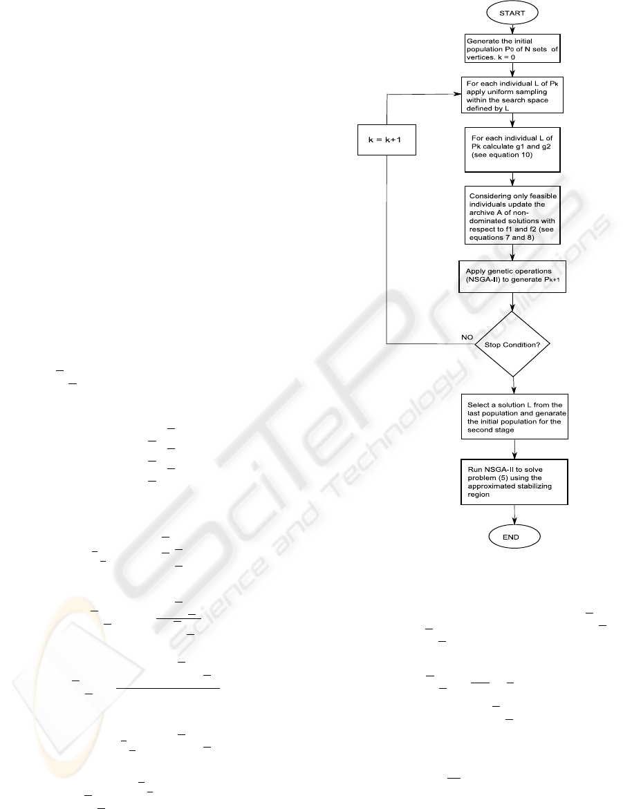
pose instead to estimate an approximation of K (see
the flowchart shown in figure 2). The proposed design
method comprises two stages. During the first stage
the goal is to calculate the vertices that maximize both
the volume of the decision space and the percent of
stable individuals. Note that these two objectives are
in conflict.
Let n be the number of decision variables for prob-
lem (5) and L, L ∈ R
n
be vectors defining the range for
each variable. As an example, for the PID problem,
we have n = 3 and
K
P
∈ [L
1
, L
1
] (9)
K
I
∈ [L
2
, L
2
]
K
D
∈ [L
3
, L
3
]
The following sub-problem is considered during
the first stage:
min
L,L∈R
n

g
1
(L, L)
g
2
(L, L)

(10)
where
g
1
(L, L) = 1 −
N
s
(L, L)
N(L, L)
(11)
g
2
(L, L) =
V
max
−
n
∏
i=1
(L
i
− L
i
)
V
max
(12)
V
max
= max
L,L∈R
n
n
∏
i=1
(L
i
− L
i
)
and
N
s
(L, L) =
N(L,L)
∑
i=1
S
t
(K
PID
i
) (13)
S
t
(K
PID
) =

0 if max
{
Re[λ(K
PID
)]
}
≥ −µ
1 otherwise
(14)
Figure 2: Flowchart of the proposed design method.
In (11) N
s
is the number of stable individuals ob-
tained via uniform sampling with boundaries L , L.
The sample size N(L , L) may be calculated using the
following Chernoff bound:
N(L, L) =
1
2ε
2
ln
2
δ
(15)
It can be shown that if N(L, L) is taken accor-
ding to (15) and the sampling is uniform the following
equation holds:
Prob





p −
N
s
N




≤ ε

≥ 1 − δ (16)
where
p = Prob
{
S
t
(K
PID
) = 1
}
(17)
We have fixed ε and δ to 0.1. Note that during
the first stage an archive of non-dominated solutions
A MULTI-OBJECTIVE APPROACH TO APPROXIMATE THE STABILIZING REGION FOR LINEAR CONTROL
SYSTEMS
155

can be updated, to be used later. In both stages any
available MOEA can be used to solve the optimiza-
tion problem. In this work we have chosen NSGA-II
(Deb et al., 2000), which is a “state of the art” multi-
objective genetic algorithm. NSGA-II is an improved
version of the original algorithm proposed in (Srini-
vas and Deb, 1994). Note that this algorithm was
previously used to design PID structures in (Lagunas,
2004). It has the following features:
• It uses an elitist principle.
• It uses and explicit diversity preserving mecha-
nism.
• There is no sharing parameter to select.
• The sorting mechanism is faster than MOGA.
The offspring is created using the parent popu-
lation and usual genetic operators. Thereafter, the
two populations are combined together and a non-
dominated sorting mechanism is used to classify the
entire population.
Special mutation and cross-over operators were
designed to generate individuals that remain within
the limits of the (approximated) feasible region.
4 NUMERICAL RESULTS
Consider the open-loop model taken from (Hohen-
bichler and Abel, 2008):
G
0
(s) =
−0.5s
4
− 7s
3
− 2s + 1
s
6
+ 11s
5
+ 46s
4
+ 95s
3
+ 109s
2
+ 74s + 24
(18)
and the filters W
n
and W
d
are defined:
W
n
(s) =
1
s + 1
,W
d
(s) = 1 (19)
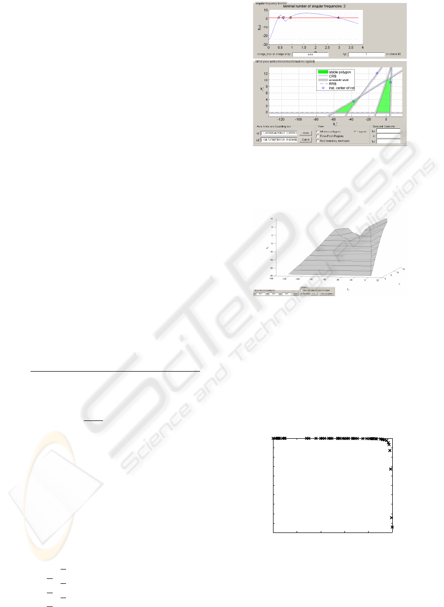
For this plant, figure 3 shows an example of the
convex stability polygons corresponding to K
P
= 1.
PIDROBUST allows also to plot the whole stabiliz-
ing region, as shown in figure 4.
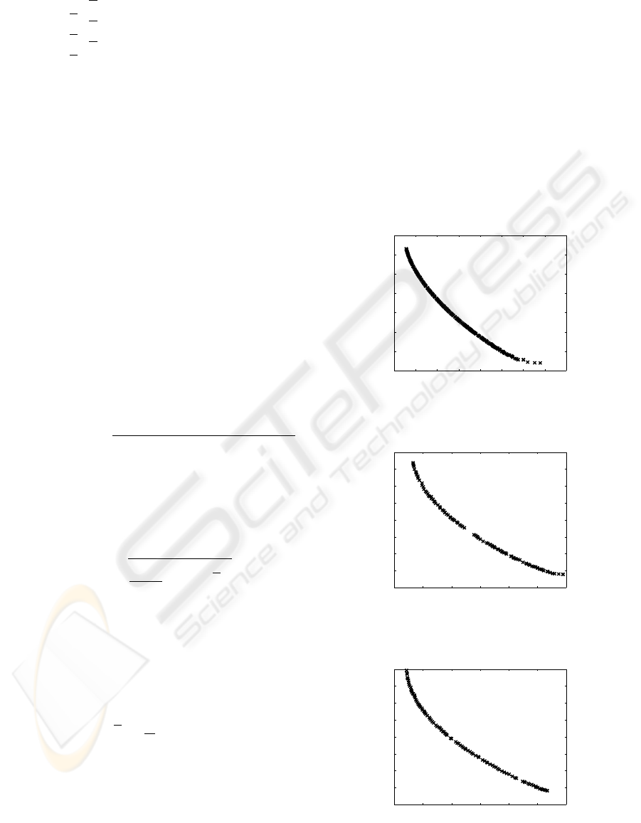
The proposed design method was coded in
MATLAB
R

7.0. Figure 5 shows a typical Pareto
approximation (Coello et al., 2007) obtained at the
end of stage 1. Note that the Pareto front approxi-
mation shows that there exist no compromise solution
between the two objectives. In this work the follow-
ing solution have been arbitrary chosen:
[L
1
, L
1
] = [−18.3, 6.1] (20)
[L
2
, L
2
] = [−4.3, 9.69]
[L
3
, L
3
] = [−83.3, 14.3]
which corresponds to g
1
≈ 0.2 and g
2
≈ 0.99.
Figure 3: Example of the convex stability polygons corre-
sponding to K
P
= 1.
Figure 4: Stabilizing region.
To compare the results, the design problem was
solved by means of the classical ”penalty function
based approach (in this case NSGA-II as a standalone
algorithm), with µ = 10
−4
, η = 10
3
, B = 10
3
and gen-
erating the individuals within the cube defined by:
K
P
, K
D
, K
I
∈ [−200, 200] (21)
0 0.2 0.4 0.6 0.8 1
0
0.1
0.2
0.3
0.4
0.5
0.6
0.7
0.8
0.9
1
g
1
g
2
Figure 5: Pareto approximation obtained at the end of the
first stage.
The comparison is fair because this region en-
velopes the true stabilizing region, although this in-
formation is not available a priori. We also include
the results corresponding to the true stabilizing region
ICINCO 2009 - 6th International Conference on Informatics in Control, Automation and Robotics
156

obtained by PIDROBUST, with boundaries:
[L
1
, L
1
] = [−22.5, 4.9] (22)
[L
2
, L
2
] = [0, 12.59]
[L
3
, L
3
] = [−118, 5.24]
Thus, three algorithms are compared:
• A1 : NSGA-II with K
P
, K
D
, K
I
∈ [−200, 200].
• A2 : NSGA-II: Stage 1 and Stage 2 (proposed new
method) with ε = 0.1 and δ = 0.1
• A3 : NSGA-II + PIDROBUST (using the true sta-
bilizing region).
Figures 6, 7 and 8 show typical approximations
obtained via A1, A2 and A3 respectively. In the
multi-objective optimization framework, there are in
general three goals (i) the distance of the resulting
nondominated set to the Pareto-optimal front should
be minimized, (ii) a uniform distribution of the solu-
tions found is desirable, and (iii) the extent of the ob-
tained nondominated front should be maximized. We
have chosen four indicators to evaluate each Pareto
approximation:
• Set Coverage (C). Given two Pareto approxima-
tions P F
1
and P F
2
, the Set Coverage is defined
as follows:
C(P F
1
, P F
2
) =
|{
b ∈ P F
2
, ∃a ∈ P F
1
: a  b
}|
|
P F
2
|
(23)
C(P F
1
, P F
2
) measures the proportion of ele-
ments in P F
2
that are dominated by at least one
element in P F
1
.
• Efficient Set Space (ESS). Defined as follows:
ESS =
s
1
N −1
N
∑
i=1
(d
i
− d)
2
(24)
Hereby, d
i
denotes the minimal Euclidean dis-
tance from the image PF
1
(x
i
) of a solution x
i
, i =
1, . . . , N, to the true Pareto front, and
d
i
:= min
j=1,...,N
i6= j
d
i j
(25)
d :=
1
N
N
∑
i=1
d
i
, (26)
where d
i j
is the Euclidean distance between
P F
1
(x
i
) and P F
1
(x
j
)
• Hypervolume (HV ). This indicator measures the
volume covered by the approximation with re-
spect to a reference point.
• Max. Distance (MD). Defined as:
MD = max
i, j=1,...,N
i6= j
d
i j
(27)
The setting used for each algorithm is shown in
table 1. Tables 2 and 3 show the indicators values for
30 executions. The mean value and the standard de-
viation (between brackets) is presented for each indi-
cator. Table 4 shows the results of Mann-Whitney-
Wilcoxon tests with a significance level α = 0.05.
Therein, the symbols =, ⇑, ⇓ mean that the algorithm
in the corresponding row is statistically equal, better
or worse than the algorithm in the column, with re-
spect to the four indicators C, ESS, HV and MD.
0.648 0.65 0.652 0.654 0.656 0.658 0.66 0.662 0.664
0.45
0.5
0.55
0.6
0.65
0.7
0.75
0.8
f
1
f
2
Figure 6: Example of Pareto approximation obtained with
algorithm A1.
0.65 0.66 0.67 0.68 0.69 0.7 0.71
0
0.1
0.2
0.3
0.4
0.5
0.6
0.7
0.8
f
1
f
2
Figure 7: Example of Pareto approximation obtained with
algorithm A2.
0.65 0.66 0.67 0.68 0.69 0.7 0.71
0
0.1
0.2
0.3
0.4
0.5
0.6
0.7
0.8
f
1
f
2
Figure 8: Example of Pareto approximation obtained with
algorithm A3.
A MULTI-OBJECTIVE APPROACH TO APPROXIMATE THE STABILIZING REGION FOR LINEAR CONTROL
SYSTEMS
157

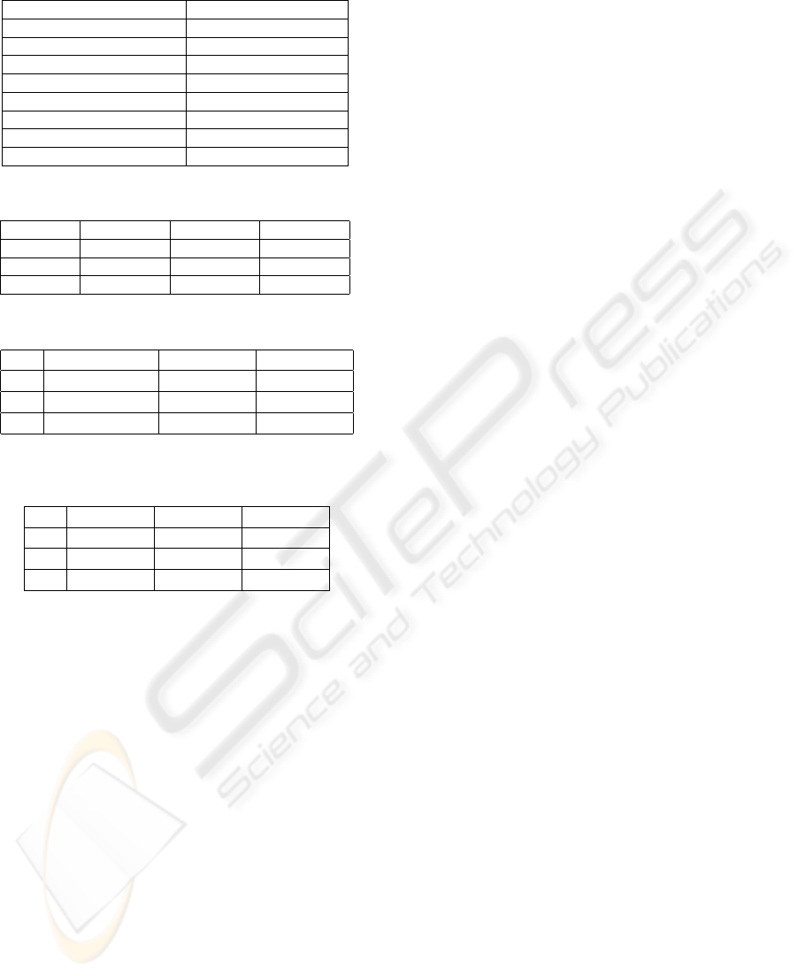
Table 1: Parameter Settings NSGA-II.
Representation Real numbers
Cross-Over Operator Uniform
Cross-Over Probability 0.9
Mutation Gaussian Perturbation
Mutation Probability 0.1
Stop Condition A1 300 generations
Selection Scheme A1 (200+200)
Stop Condition A2,A3 50 generations
Selection Scheme A2,A3 (100+100)
Table 2: Results for the coverage indicator.
C(A
i
, A
j
) A1 A2 A3
A1 − 0.26(0.31) 0.23(0.33)
A2 0.26(0.43) − 0.20(0.33)
A3 0.23(0.39) 0.56(0.35) −
Table 3: Results for indicators ESS, HV and DMAX.
ESS HV MD
A1 0.0452(0.05) 0.03(0.03) 0.03(0.03)
A2 0.14(0.08) 0.13(0.00) 0.15(0.09)
A3 0.11(0.07) 0.10(0.02) 0.11(0.07)
Table 4: Results for Mann-Whitney-Wilcoxon tests with a
significance level α = 0.05.
A1 A2 A3
A1 − =, ⇑, ⇓, ⇓ =, ⇑, ⇓, ⇓
A2 =, ⇓, ⇑, ⇑ − ⇓, ⇓, ⇑, ⇓
A3 =, ⇓, ⇑, ⇑ ⇑, ⇑, ⇓, ⇑ −
5 CONCLUSIONS
In this paper a new design method for solving multi-
objective control problems was described. Results
show that, for the PID control problem, the proposed
method (A2) is able to find better approximations than
the conventional method (A1) with respect to the HV
and MD indicators, given the same number of func-
tions evaluations. Moreover, when compared to A3
(the algorithm using the true stabilizing region), re-
sults show that A2 is indeed able to find a good ap-
proximation of the feasible region.
In the future the authors will try to extend this
work, in order to consider more complex control
problems, with more design variables and objectives.
For that goal, a more sophisticated representation of
the search space is needed (stage 1), in order to make
the sampling process more efficient.
REFERENCES
Arakawa, M., Nakayama, H., Hagiwara, I., and Yamakawa,
H. (1998). Multiobjective Optimization Using Adap-
tive Range Genetic Algorithms with Data Envelop-
ment Analysis. In A Collection of Technical Papers
of the 7th Symposium on Multidisciplinary Analysis
and Optimization, pages 2074–2082.
Calafiore, G. and Dabbene, F. (2006). Probabilistic and
Randomized Methods for Design under Uncertainty.
Springer-Verlag,London.
Coello, C., Lamont, G., and Van-Veldhuizen, D. (2007).
Evolutionary Algorithms for Solving Multi-Objective
Problems. Springer.Genetic and Evolutionary Com-
putation Series.Second Edition.
Deb, K., Agrawal, S., Pratab, A., and Meyarivan, T. (2000).
A Fast Elitist Non-Dominated Sorting Genetic Algo-
rithm for Multi-Objective Optimization: NSGA-II. In
Proceedings of the Parallel Problem Solving from Na-
ture VI Conference, pages 849–858.
Fleming, P. (2001). Genetic Algorithms in Control System
Engineering. Technical report, Research Report No.
789. University of Sheffield.UK.
Herreros, A. (2000). Diseo de controladores robustos mul-
tiobjetivo por medio de algoritmos geneticos. Tesis
Doctoral, Departamento de Ingenieria de Sistemas y
Automatica.Universidad de Valladolid, Espana.
Hohenbichler, N. and Abel, D. (2008). Calculating All KP
Admitting Stability of a PID Control Loop. In Pro-
ceedings of the 17th World IFAC Congress. Seoul, Ko-
rea, July 6-11, pages 5802–5807.
Khor, E., Tan, K., and Lee, T. (2002). Learning the Search
Range for Evolutionary Optimization in Dynamic En-
vironments. Knowledge and Information Systems Vol.
4 (2), pages 228–255.
Lagunas, J. (2004). Sintonizacin de controladores PID
mediante un algoritmo gentico multi-objetivo (NSGA-
II). PhD thesis, Departamento de Control Automtico.
Centro de Investigacin y de Estudios Avanzados. Mx-
ico.
Michalewicz, Z. (1995). A survey of constraint handling
techniques in evolutionary computation methods. In
Proceedings of the 4th Annual Conference on Evolu-
tionary Programming, pages 135–155. MIT Press.
Sasaki, D., Obayashi, S., and Nakahashi, K. (2002). Navier-
Stokes Optimization of Supersonics Wings with Four
Objectives Using Evolutionary Algorithms. Journal
of Aircraft, Vol. 39, No. 4, 2002, pp. 621629.
Srinivas, N. and Deb, K. (1994). Multiobjective Optimiza-
tion Using Nondominated Sorting in Genetic Algo-
rithms. Evolutionary Computation. Vol 2. No 3, pages
221–248.
Tan, K., Khor, E., and Lee, T. (2005). Multiobjective
Evolutionary Algorithms and Applications. Springer-
Verlag.
ICINCO 2009 - 6th International Conference on Informatics in Control, Automation and Robotics
158