AN ANALYTICAL AND NUMERICAL STUDY
OF PRESSURE TRANSIENTS IN PNEUMATIC
DUCTS WITH FINITE VOLUME ENDS
N. I. Giannoccaro, A. Messina and G. Rollo
Dipartimento di Ingegneria dell’Innovazione, Università del Salento, Via per Monteroni, Lecce, Italia
Keywords: Industrial automation, Pneumatic transmission line, Finite volumes, Ducts, Fluid mechanics.
Abstract: In this paper, the response of a pneumatic transmission line is analysed through two different approaches.
Both the approaches, based on the same physical model, are able to simulate the dynamics of a pneumatic
line, with finite volume ends. The first approach analytically provides the transients through an equation in a
quasi-closed form; the second approach is based on a numerical procedure yielding the inversion of the
Laplace transform by the application of a trapezoidal rule. The analysis of the mutual performances of the
two approaches, in the frame of pneumatic systems normally operating in industrial automation, can be
useful in terms of control of the response and could assist in the design of pneumatic systems.
1 INTRODUCTION
Pneumatic actuators are often employed in industrial
automation for reasons related to their good power/
weight ratio, easy maintenance and assembly
operations, clean operating conditions and low cost.
This set of advantages, however, is negatively
balanced by the difficulties met during the design.
Indeed, the presence of air, along with its natural
compressibility, introduces further complexities to
those already existing: friction forces, losses and
time delays in cylinder and transmission lines
(Messina, 2005), (Carducci, 2006). For these
reasons, fast transients involved in wave
propagations in pneumatic transmission lines
deserve to be taken into account in the design of the
system (Rollo, 2007).
The pneumatic transmission line, analysed in this
work, consists of a tube, of a certain length,
connecting two finite capacities. As far as the gas-
dynamic inside the duct is concerned, in literature
there are several papers dealing with such systems
but only describing lines with one of the two
capacities being finite. In this work, the
mathematical description of a pneumatic line, with
finite volume terminations, is presented. This setting
complicates the mathematics of the phenomena but
it is interesting because of the industrial practice
(Messina, 2005), (Rollo, 2007) where finite
capacities are very common. The transient in the line
is described through two partial differential
equations, whose solution is obtained in
correspondence to suitable initial and boundary
conditions. The mathematical model (Rollo, 2007)
gives the pressure response for a double volume
terminated pneumatic line and includes as a
particular case a previous model presented by
Schuder and Binder (Schuder, 1959).
The model is obtained assuming small pressure
and temperature changes, such that the following
assumptions are valuable (Schuder, 1959): (i)
incompressible flow and (ii) laminar flow; the
accuracy of the response, in correspondence of
different operative conditions, has been discussed
elsewhere (Rollo et al., 2007).
The assumptions of the model mainly concern
the flow conditions which allow an approach based
on the Laplace transform (Rollo, 2007), (Schuder,
1959). This type of model could be considered
attractive in the frame of industrial automation, but a
possible difficulty arises in the inverse
transformation especially when an analytical
description of the transient is attempted (Rollo,
2007). In this respect, a numerical method (Crump,
1976), (Duffy, 1993), that readily determines the
Laplace transform inversion, could be considered
attractive in order to achieve the pressure transient.
These two approaches, the analytical one (Rollo,
2007) and the numerical one (Duffy, 1993), that
60
I. Giannoccaro N., Messina A. and Rollo G.
AN ANALYTICAL AND NUMERICAL STUDY OF PRESSURE TRANSIENTS IN PNEUMATIC DUCTS WITH FINITE VOLUME ENDS.
DOI: 10.5220/0002169000600066
In Proceedings of the 6th International Conference on Informatics in Control, Automation and Robotics (ICINCO 2009), page
ISBN: 978-989-674-001-6
Copyright
c
 2009 by SCITEPRESS – Science and Technology Publications, Lda. All rights reserved

have different complexities, are taken into account
herein. The first analytically provides the description
of the pressure transients through an equation in a
quasi-closed form. The second is numerically able to
yield the inversion of the Laplace transform in a
direct way, through a trapezoidal rule (Crump,
1976), (Duffy, 1993). This latter, under certain
conditions, requires no manipulation on Laplace
transform.
The two approaches, with the analysis of the
mutual performances, can suggest, in the frame of
pneumatic systems normally operating in industrial
automation, the strategies in terms of design and
control of the response. In this respect, interesting
conclusions can be extracted.
2 SYSTEM ANALYSED
For a self comprehension of the present work, a brief
description of the real system analysed is also
presented. The relevant physical model which is
referred to in the present work is illustrated in Fig. 1.
The system under investigation consists of two
chambers having volumes Q
1
, Q
2
. The chambers are
connected through a cylindrical tube (also termed as
pneumatic transmission line) whose transversal
section is constant in the range of commercial
tolerances. The x-longitudinal coordinate is settled
from the upstream (chamber 1: Q
1
) to the
downstream chamber (chamber 2: Q
2
).
The upstream chamber consists of a five litre
tank arranged with four holes in order to allow the
external connections. In particular, chamber 1 is
filled up through a tap air supply until an established
static pressure, measured by the absolute pressure
gage, is reached. An airtight adapter is screwed onto
chamber 1. The adapter is made airtight through an
internal membrane made of commercial sticky tape.
The test and simulated condition consists of
suddenly breaking the membrane in order to allow a
wave pressure travel from chamber 1 to chamber 2
and vice versa; the sudden rupture of the membrane
is caused by a puncturing actuator placed at the
symmetrical end with respect to the membrane; the
puncturing actuator is quasi-statically activated by
manually pushing its rod through orifice A.
When a step pressure signal propagates through
the duct an on/off valve can be considered simulated
(Rollo, 2007). Based on these motivations the
approaches (analytical and numerical) have been
tested with respect to the mentioned step-type signal.
The downstream volume consists of the ram
chamber of a commercial double acting pneumatic
actuator. The established volume Q
2
can be in
practice settled by grounding the rod of the actuator
at a fixed position.
Figure 1: Scheme and nomenclature of the system.
3 SCHUDER AND BINDER
EXTENDED (SBE) MODEL:
ANALYTICAL APPROACH
In the SBE model (Rollo, 2007), (Schuder, 1959),
the equation describing the pressure transient in the
duct, obtained from an analytical solution of two
partial differential equations (one-dimensional mass
and momentum conservation law (Schuder, 1959)),
is obtained using the Laplace transform.
This kind of procedure yields, in the Laplace
domain and in correspondence of an established
section of the line (x=L), the following response:
()
() ()
()
s
p
βLsinhQkQ
a
β
β
a
βLcoshQkQ
1
kQ
s
pp
sL;P
0
21
21
1
0m
+
⎥
⎥
⎥
⎥
⎦
⎤
⎢
⎢
⎢
⎢
⎣
⎡
⎟
⎟
⎠
⎞
⎜
⎜
⎝
⎛
+
++
⋅⋅
⎟
⎠
⎞
⎜
⎝
⎛
−
=
(1)
where a is the cross sectional area of the duct, k the
ratio of specific heats at pressure and volume
constant (c
p
/c
v
), L the length of the duct, p
m
and p
0
the initial pressure in the sending volume and
connecting duct respectively, Q
1
and Q
2
the sending
and receiving volume respectively and β is the
following parameter:
(
)
2
ρc
ρsRs
β
+
=
(2)
depending on R (frictional resistance in duct in the
presence of laminar flow), s the Laplace variable, ρ
the density (constant) and c the sound speed
(constant).
AN ANALYTICAL AND NUMERICAL STUDY OF PRESSURE TRANSIENTS IN PNEUMATIC DUCTS WITH
FINITE VOLUME ENDS
61

The inverse transform of (1) is not a
straightforward task; in this respect, following
Schuder and Binder, Jaeger’s result is taken into
account (Schuder, 1959): evaluating the coefficients
of an exponential series, it is possible to obtain the
following analytical solution showing the pressure in
the time domain in the position close to chamber 2
(x=L):
()
()
()
∑
∞
=
−
⎥
⎥
⎥
⎥
⎥
⎦
⎤
⎢
⎢
⎢
⎢
⎢
⎣
⎡
⎟
⎟
⎠
⎞
⎜
⎜
⎝
⎛
−
+
⎟
⎟
⎠
⎞
⎜
⎜
⎝
⎛
+++
⎥
⎦
⎤
⎢
⎣
⎡
⎟
⎠
⎞
⎜
⎝
⎛
+
⎟
⎠
⎞
⎜
⎝
⎛
⋅
⋅−−
++
++
=
1n
n
1n
n2
n
1
2
n
2
1
2
n
n
n
n
2ρ
Rt
0m
21
201m
A
cosα
kQα
aL
aL
αQ
sinα
kQα
aL
aL
Q
kQ
Q
1
α
2
t
sin
ρ
R
2
t
cos
epp2
aLQkQ
aLQpkQp
tL;P
ϑ
ϑ
ϑ
(3)
where t is the time; α
n
and θ
n
are functions of the
geometry of the line and initial flow conditions; in
particular, the poles in Equation (1) are function of
α
n
too (Rollo, 2007), (Schuder, 1959). In fact, by
substituing in Equation (1)
()
iα
ρc
ρsRs
LβL
2
1
2
=
⎟
⎟
⎠
⎞
⎜
⎜
⎝
⎛
+
=
(4)
and equating to zero the common denominator of
Equation (1), an implicit equation in α is obtained;
once it is solved (numerically, with the Newton-
Raphson method), after some simple mathematical
manipulations, it is possible to obtain, along with
s
0
=0 (Rollo, 2007), (Schuder, 1959):
2
2
n
n
ρ
R
L
c2α
2
i
2ρ
R
s
⎟
⎟
⎠
⎞
⎜
⎜
⎝
⎛
−
⎟
⎠
⎞
⎜
⎝
⎛
±−=
(5)
in which the real part of the poles is negative or
zero.
The quasi-closed form solution (3) depends on
the number of the terms in the series; the only non-
serious drawback is the necessity of resorting to a
numerical method in order to assess α
n
. Equation (3)
yields p(L;t) for a double volume terminated
pneumatic line and it is an extension of a previous
model presented by Schuder and Binder (Schuder,
1959). The analytical approach to the SBE model is
one of the most complete treatments among those
presented about transients in pneumatic lines within
relevant literature, in which the influence of pressure
waves propagating in ducts is, sometimes, neglected
or poorly described. Furthermore, even if it is
obtained using the following assumptions: (i)
incompressible flow and (ii) laminar flow, it can be
adopted, without significantly reducing the accuracy
of the response, in correspondence to certain
operative conditions (Rollo et al., 2007), where the
relevant investigations showed its ability to describe
pressure transients including reflecting waves.
4 NUMERICAL APPROACH
The Jaeger’s results, in the SBE model, are related to
the fact that the solution (3) depends i) on the
numerical evaluation of α
n
and ii) on a certain
amount of labor for the mathematical procedure
leading to Equation (3) in the inverse Laplace
transform (Rollo, 2007), (Schuder, 1959). A kind of
resolution allowing to obtain the inverse transform
of Equation (1) in a direct way, could be considered
attractive in the frame of systems normally operating
in industrial automation. In this respect the authors
suggest, in this work, to solve the problem of readily
determining the inverse Laplace transform using a
numerical approach. Within relevant literature, a
large number of different methods for numerically
inverting the Laplace transform have been
introduced and tested: one of these uses a Fourier
series approximation (Crump, 1976), (Duffy, 1993).
In fact, in (Duffy, 1993) the following
straightforward application of a trapezoidal rule in
order to provide the numerical inversion of Laplace
transform (here referred to Eq. (1)) is proposed:
()
()
[]
()
()
⎪
⎪
⎪
⎪
⎭
⎪
⎪
⎪
⎪
⎬
⎫
⎪
⎪
⎪
⎪
⎩
⎪
⎪
⎪
⎪
⎨
⎧
⎥
⎥
⎥
⎥
⎥
⎦
⎤
⎢
⎢
⎢
⎢
⎢
⎣
⎡
⎥
⎦
⎤
⎢
⎣
⎡
⎟
⎠
⎞
⎜
⎝
⎛
−
+
+
⎥
⎦
⎤
⎢
⎣
⎡
⎟
⎠
⎞
⎜
⎝
⎛
+
−
+
=
∑
∞
=1z
z
μt
2t
πi12z
μL;PIm
t
i πz
μL;PRe
1
μL;PRe
2
1
2t
e
tL;P
(6)
where t is the time, i the imaginary unit, Im and Re
indicate the imaginary and real part of the quantity
in the brackets respectively and μ must be greater
than the real part of any singularity (poles) in P(L;s)
(Duffy, 1993).
The accuracy and efficiency of such a numerical
approach depend on a suitable choice of some
parameters. In particular, μ can be evaluated
through certain considerations about the
discretization error (related to the step size π/t for
ICINCO 2009 - 6th International Conference on Informatics in Control, Automation and Robotics
62

the trapezoidal rule) deriving from the application of
Eq. (6). Following the approach proposed in
(Crump, 1976), introducing the hypothesis that the
function of interest is bounded by:
()
λt
MetL;P ≤
(7)
(with M and λ real numbers) it is possible to choose
μ through the following relation:
(
)
2
t
Errln
λμ −=
(8)
where Err is the error parameter within the
numerical accuracy desired and the parameter λ can
be chosen slightly larger than the maximum of the
real part of all the poles (Crump, 1976). Once μ is
known, the series (6) can be summed until it
converges to the desired number of significant
figures (Crump, 1976). Usually the series in (6) can
converge slowly (this has been observed in some
tests not reported here); furthermore, (Crump, 1976)
the use of a sequence accelerator in conjunction with
the numerical inversion is recommended, also in
order to obtain a reduction of the truncation error
(indeed the series in Eq. (6) is not summed to
infinity). In this case, following the considerations in
(Crump, 1976), (Duffy, 1993), here Wynn’s epsilon-
algorithm is adopted. More specifically, to
accelerate the convergence of the sequence of partial
sums in (6) using the epsilon-algorithm, it is possible
to calculate them as in (9):
() []
()
()
1.1,...,2Nz
,
2t
πi12z
μL;PIm
t
i πz
μL;PRe
1SS
,μL;PRe
2
1
S
z
1zz
0
+=
⎥
⎥
⎥
⎥
⎥
⎦
⎤
⎢
⎢
⎢
⎢
⎢
⎣
⎡
⎥
⎦
⎤
⎢
⎣
⎡
⎟
⎠
⎞
⎜
⎝
⎛
−
+
+
⎥
⎦
⎤
⎢
⎣
⎡
⎟
⎠
⎞
⎜
⎝
⎛
+
−+=
=
−
(9)
It is possible, then, to define ε
-1
(m)
=0, ε
0
(m)
=S
m
,
m=0, 1,..,2N and then put:
() () () ()
[]
0,...,2Np
,εεεε
1
m
p
1m
p
1m
1p
m
1p
=
−+=
−
++
−+
(10)
In this way, the sequence ε
0
(0)
, ε
2
(0)
, ε
4
(0)
,.., ε
2N
(0)
gives better successive approximation to the sum of
the series (Crump, 1976). So, Equation (6),
including the sequence accelerator, becomes
Equation (11):
()
() 0
2N
μt
NUM
ε
2t
e
tL;P ⋅=
(11)
5 ANALYTICAL VS NUMERICAL
APPROACH: CONDITIONS,
RESULTS AND DISCUSSIONS
The analytical approach presented in Section 3
(Rollo, 2007) was used for an interesting
comparison, with respect to a more refined model
NLC (for Non Laminar Compressible flow) (Rollo,
2007), (Rollo et al., 2007). This latter model, whose
behaviour was validated through experimental
investigations (Rollo, 2007) on the physical model
of Fig. 1, takes into account i) flow not necessarily
laminar and ii) compressible flow. Through a
suitable error parameter, the discrepancy on the
response of a pneumatic line with established
geometrical characteristics (L=2.53m, D=3 or 6 mm,
Q
1
= 5dm
3
), for polyurethane ducts with an assumed
internal roughness of 3μm (Rollo, 2007) was
estimated for various flow conditions. In both
models, the relevant solution can be obtained and
displayed, in space (at a fixed time) and in time (at a
fixed position); however, the major relevance of the
performance in industrial applications (Messina,
2005), (Rollo, 2007) is related to the behaviour of
the pressure in the ram chamber of the actuator
(x=L). Therefore, only p(L;t) was discussed, in
correspondence of the various receiving volumes Q
2
(obtained fixing the stroke of the pneumatic actuator
employed as downstream volume, in correspondence
of different positions).
This comparison highlighted that, for a fixed
geometrical configuration, the error between the
SBE and NLC models is as small as the pressure
ratio p
m
/p
o
is close to 1 (Rollo, 2007); in this case
the match of SBE response with the NLC curve is
very satisfactory. This comparison was made after
appropriate convergence tests, that suggested to use
n=0,…..,30 in the Equation (3) for the SBE model.
In this work, the comparison between the
analytical (3) and numerical (11) approach is
discussed, in correspondence of some settings
yielding a satisfactory agreement of the SBE with
the NLC model. In particular, a line with L=2.53m,
D=3 mm and Q
1
= 5dm
3
will be considered. The case
of interest concerns the transient caused by an
AN ANALYTICAL AND NUMERICAL STUDY OF PRESSURE TRANSIENTS IN PNEUMATIC DUCTS WITH
FINITE VOLUME ENDS
63

upstream initial pressure in Q
1
of 1.1 times higher
than initial atmospheric pressure. This setting is
completed arranging the actuator employed as
downstream volume to establish, in a first case, a
volume Q
2
= 1.5 cm
3
(capacity corresponding to the
dead space of the ram chamber) and, in a second
case, Q
2
= 26.5 cm
3
(Rollo, 2007).
A suitable error parameter is introduced (12) for
the detection of discrepancy of the two approaches
(3) and (11):
() ()
()
A
NUMA
tL;p
tL;ptL;p
ERROR
−
=
(12)
in correspondence to various values of the time (10
ms≤t≤150 ms). In applying (11), it is assumed
Err=10
-6
and, for the considerations about Eqs. (5)
and (8), it can be assumed λ=0. In this way, the μ
value is known in all the time instants considered.
The comparison will be made firstly assuming, as far
as the numerical approach (11) is concerned, N=25.
In this respect, for the first case (Q
2
=1.5 cm
3
) the
following Table 1 was produced:
Table 1: Simulated Pressure with L=2.53 m, D=3 mm,
p
m
/p
0
=1.1, Q
2
=1.5 cm
3
(n=30, N=25).
Time Instants
(ms)
Analytical
Pressure
(bar)
Numerical
Pressure
(bar) ERROR
10 1.092289 1.092282 6.8E-06
20 1.116303 1.116265 3.4E-05
30 1.101538 1.101535 2.1E-06
40 1.097992 1.097992 3.5E-08
50 1.099557 1.099561 3.7E-06
60 1.099927 1.099927 1.5E-07
70 1.099681 1.099659 1.9E-05
80 1.099693 1.099693 1.7E-07
90 1.099725 1.099726 2.8E-07
100 1.099725 1.099726 1.1E-07
110 1.099723 1.099723 1.1E-07
120 1.099724 1.099724 2.9E-09
130 1.099724 1.099724 1.5E-08
140 1.099724 1.099724 4.5E-09
150 1.099724 1.099724 4.4E-10
Pressure
computational
time (ms) ~ 5 ~ 290
In Table 1 the first column shows the time
instants taken into account, the second and third
columns show the pressure values obtained with the
two approaches, the analytical one and the numerical
one respectively, the fourth column shows the
ERROR values. Table 1 shows an agreement of the
analytical and numerical results (second and third
column) that can be considered very satisfactory;
furthermore, it is possible to notice that the
computational times (evaluated on a 2.8 GHz
Pentium IV using a Matlab routine) show that the
analytical approach needs about 5 ms to provide the
pressure values in the second column, whilst the
numerical computational time is about 290 ms.
As far as the second case (Q
2
=26.5 cm
3
) is
concerned, the following Table 2 was produced:
Table 2: Simulated Pressure with L=2.53 m, D=3 mm,
p
m
/p
0
=1.1, Q
2
=26.5 cm
3
(n=30, N=25).
Time Instants
(ms)
Analytical
Pressure
(bar)
Numerical
Pressure
(bar) ERROR
10 1.018830 1.018831 3.6E-07
20 1.053451 1.053449 2.1E-06
30 1.076250 1.076250 1.6E-08
40 1.087726 1.087726 1.9E-08
50 1.093537 1.093539 1.6E-06
60 1.096557 1.096557 9.1E-09
70 1.098006 1.098006 3.3E-08
80 1.098703 1.098703 2.0E-07
90 1.099047 1.099047 5.3E-09
100 1.099214 1.099214 1.6E-07
110 1.099294 1.099293 1.1E-06
120 1.099333 1.099333 5.3E-12
130 1.099352 1.099352 5.9E-09
140 1.099361 1.099361 1.4E-09
150 1.099366 1.099366 1.9E-10
Pressure
computational
time (ms) ~ 5 ~ 290
Table 2 is also able to show a satisfactory
agreement of the results of the two approaches (3)
and (11) and, as in Table 1, it is possible to notice
that the numerical computational time is about 290
ms, whilst the analytical approach needs about 5 ms
to provide the pressure values in all the time instants
considered.
Table 1 and Table 2 can suggest that the
numerical approach (11) is not always advisable in
engineering applications in which the performance is
required in terms of design and fast control of the
response. A possible way to highlight this drawback
can be based on the study of the discrepancies with
the analytical approach, decreasing N in such a way
as to reduce the computational time of the numerical
approach (like in Table 3). In Table 3, the first
column shows the operative conditions taken into
account, the second column the mean of ERROR
values and the third the numerical computational
times. As can be seen, the computational times
decrease if N decreases, but this behaviour still
ICINCO 2009 - 6th International Conference on Informatics in Control, Automation and Robotics
64

seems far from the more attractive computational
times of the analytical approach. Furthermore
decreasing the value of N, the mean ERROR value
slightly increases.
Table 3: ERROR for a pneumatic line with L=2.53 m,
D=3 mm, p
m
/p
0
=1.1, Q
2
=1.5 cm
3
and Q
2
=26.5 cm
3
, n=30.
Mean of
ERROR
values
Numerical
computational
times (ms)
N=25
Q
2
=1.5 cm
3
4.4E-6 290
N=25
Q
2
=26.5 cm
3
3.8E-7 290
N=20
Q
2
=1.5 cm
3
2.4E-5 204
N=20
Q
2
=26.5 cm
3
7.2E-7 204
N=10
Q
2
=1.5 cm
3
6.4E-5 77
N=10
Q
2
=26.5 cm
3
7.6E-6 77
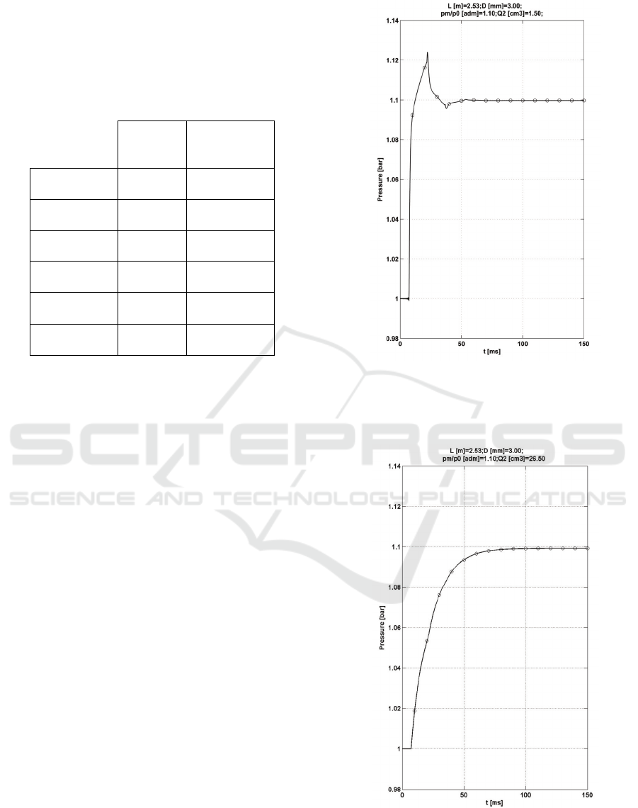
An estimation of the behaviour of both
approaches concerning the transient in the
aforementioned pneumatic lines, can be obtained
through the following Fig. 2 and Fig. 3, useful also
in order to estimate the pressure transients of Eq. (3)
and Eq. (11) in terms of design of the line.
Finally, also Figure 4 has been produced. This
latter figure has been introduced with the motivation
of showing the satisfactory agreement of both the
proposed approaches, also in correspondence of an
intermediate receiving volume (Q
2
=16.5 cm
3
).
6 CONCLUSIONS
In this paper, two approaches of different
complexities, concerning the dynamics of a
pneumatic transmission line with finite volume ends,
have been analysed: one analytical and another one
numerical. The first one provides the description of
the pressure transients through an equation in a
quasi-closed form and gives the pressure response
for a double volume terminated pneumatic line.
Figure 2: Simulated pressure at the receiving volume
through analytical (__) and numerical (°) approach with
D=3mm, L=2.53m, p
m
/p
0
=1.1 and Q
2
=1.5cm
3
(n=30,
N=25).
Figure 3: Simulated pressure at the receiving volume
through analytical (__) and numerical (°) approach with
D=3mm, L=2.53m, p
m
/p
0
=1.1 and Q
2
=26.5cm
3
(n=30,
N=25).
AN ANALYTICAL AND NUMERICAL STUDY OF PRESSURE TRANSIENTS IN PNEUMATIC DUCTS WITH
FINITE VOLUME ENDS
65

Figure 4: Simulated pressure at the receiving volume
through analytical (__) and numerical (°) approach with
D=3mm, L=2.53m, p
m
/p
0
=1.1 and Q
2
=16.5cm
3
(n=30,
N=25).
The second, numerically, is able to yield the
inversion of the Laplace transform through a
trapezoidal rule (in conjunction with a sequence
accelerator). Using certain geometrical
configurations and flow conditions, for which it was
shown that the SBE model can be used without
significantly reducing the accuracy of the response,
the two kinds of resolution can be compared and
analysed. The introduction of a suitable error
parameter, able to provide the discrepancies of the
two approaches, allows interesting discussions.
The trapezoidal rule, in its numerical simplicity,
could avoid the long mathematical procedures
yielding the inversion of the Laplace transform. The
advantage related to the application of this direct
rule seems, however, negatively balanced by the
extra computational efforts required to achieve a
satisfactory convergence (the series approximation
can converge slowly and, usually the use of a
sequence accelerator in conjunction with the
numerical inversion is highly recommended). For
these reasons, the numerical approach could not
always be advisable in engineering applications in
which performances are required in terms of design
and control of the response. This, indeed, has been
showed by the comparison with an analytical
solution in a quasi-closed form, in terms of
computational times. The possible drawback of this
latter approach is a verbose procedure giving the
final relation and the need to resort to a numerical
method in order to assess all the poles involved in
the Laplace transform. However, the relevant
simulations carried out highlight an excellent
behaviour of the analytical approach: these
properties can be considered attractive also
considering the satisfactory overlap of the curves
provided by the analytical approach with a more
performing numerical model (NLC), whose
excellence has been confirmed with experimental
validations.
The study presented in this paper gives the
possibility of investigating relevant dynamic
behaviours, suggesting an efficient estimation of
control and design parameters, in the frame of
systems normally operating in industrial automation.
REFERENCES
Messina, A., Giannoccaro, N. I., Gentile, A., 2005.
Experimenting and modelling the dynamics of
pneumatic actuators controlled by the pulse width
modulation (PWM) technique. Mechatronics, 15, 859-
881.
Carducci, G., Giannoccaro, N. I., Messina, A., Rollo, G.,
2006. Identification of viscous friction coefficients for
a pneumatic system model using optimization
methods. Mathematics and Computers in Simulation,
71, 385-394.
Rollo, G., 2007. Analisi dinamiche di tipici sistemi
meccanici ad attuazione pneumatica. Ph. D. Thesis,
Università del Salento, Dipartimento di Ingegneria
dell’Innovazione, Lecce.
Schuder, C.B., Binder, R.C., 1959. The response of
pneumatic transmission lines to step inputs. Trans.
ASME, 81, 578-584.
Rollo, G., Messina, A., Gentile, A., 2007. Influence of
geometrical parameters and operative conditions on
pressure transients in pneumatic ducts. XVIII
Congresso AIMETA di Meccanica Teorica e
Applicata, MA 15, 453.
Crump, K. S., 1976. Numerical inversion of Laplace
transforms using a Fourier series approximation.
Journal of the Association for Computing Machinery,
23, 89-96.
Duffy, D. G., 1993. On the numerical inversion of Laplace
transforms: comparison of three new methods on
characteristic problems from application. ACM
Transaction on Mathematical Software, 19, 333-359.
ICINCO 2009 - 6th International Conference on Informatics in Control, Automation and Robotics
66