Performance Assessment of Patch-based Bilateral

Denoising

Arnaud de Decker

, John Aldo Lee

and Michel Verleysen

Machine Learning Group, Universit

e catholique de Louvain

pl. du Levant 3, 1348 Louvain-la-Neuve, Belgium

Molecular Imaging and Experimental Radiotherapy StLuc University Hospital

Universit

e Catholique de Louvain, av. Hippocrate 54, 1200 Bruxelles, Belgium

Abstract. In the ﬁeld of medical image analysis, denoising is one of the most

important preprocessing steps before medical analysis. The design of an efﬁ-

cient, robust, and computationally effective edge-preserving denoising algorithm

is a widely studied, and yet unsolved problem. One of the most efﬁcient edge-

preserving denoising algorithms is the bilateral ﬁlter, which is an intuitive gener-

alization of the local M-smoother. In this paper, we propose to modify both the

bilateral ﬁlter and the local M-smoother to use patches of the image instead of

single voxels in the denoising process. Using patches instead of single voxels in

the ﬁltering process is a way to adapt the ﬁlter to the textures, ramps, and edges

of the image, and make the ﬁlter more discriminant. The ﬁltering performances

of the patch-based algorithms are evaluated on a benchmark and a CT phantom

image and compared to the bilateral ﬁlter and local M-smoother.

1 Introduction

Nowadays, medical images are essential tools for medical doctors. They are used in ra-

diotherapy, nuclear medicine, radiology, oncology, and many other ﬁelds of medicine.

However, they are often polluted by noise and blur. These problems can induce misin-

terpretations and lead to errors in diagnosis and treatment. For example, in radiotherapy,

it is of crucial importance to have a precise identiﬁcation of the volumes to be treated.

For this reason, the ﬁrst and more important preprocessing step after the acquisition of

a medical image is to use a ﬁltering algorithm in order to get rid of the noise before the

actual analysis.

In denoising methods, the challenge is to obtain a ﬁltering effect powerful enough

to remove most of the noise generated during the acquisition process while preserving

the edges and textures in the image. This problem becomes even more complicated

for medical images as they often have a relatively low resolution. Furthermore, a ﬁlter

which does not preserve edges accurately blurs the image, which reduces the resolution

even more.

Several algorithms have been used for unsupervised edge-preserving denoising of

medical images: wavelet transform [1], [2], partial differential equations [3], total vari-

ation [4], Bayesian denoising [5], kernel regression [6], gradient approximation [7] ,

de Decker A., Aldo Lee J. and Verleysen M. (2009).

Performance Assessment of Patch-based Bilateral Denoising.

In Proceedings of the 1st International Workshop on Medical Image Analysis and Description for Diagnosis Systems, pages 52-61

DOI: 10.5220/0001813900520061

 SciTePress

local M-smoother [8], [9], bilateral [10], [11], or even trilateral ﬁltering [12]. Kervrann

also used patch based algorithms [13], [14] for denoising purposes.

Among these algorithms, the bilateral ﬁlter (BF) and the local M-smoother (LMS)

have been quite popular lately because of their intuitive formulation, their low compu-

tational load, and their efﬁciency in terms of edge-preserving denoising performances.

Still, while the BF and LMS algorithms are excellent for piecewise constant images

denoising, their performances drop signiﬁcantly when the image is blurred or contains

ramps, which is the case in most realistic situations. Indeed, these algorithms are based

on the principle of mode identiﬁcation. When the image is not piecewise constant, there

is no mode to identify and the ﬁlters become less efﬁcient.

In this paper, we propose to generalize the BF algorithm to use subsets of adjacent

voxels of the image, called patches, instead of single voxels. As these patches are com-

posed of more than one voxel and gather information in 2 or 3 dimensions around their

center, the ﬁltering becomes more selective and the performance of this patch-based

bilateral ﬁltering (PBBF) improves.

The rest of this paper are organised as follows. In Section 2 we will deﬁne the image

model, and brieﬂy introduce the local M-smoother and the bilateral ﬁlter algorithms.

Then, we will describe how patches are introduced in these classical algorithm. The

benchmark image we used to test the ﬁltering performances in this paper is introduced

in Section 3 with a comparison of the performances and visual results of the algorithm

with state-of-the art BF and LMS. Finally, Section 4 gathers the conclusions and future

perspectives.

2 Image Model and Patch-based Bilateral Filter

2.1 Image Model

Let us deﬁne a D-dimensional image as a vector of voxels in which the i

voxel position

can be uniquely identiﬁed by vector x

= (x

, . . . , x

). The voxel at coordinate x

has

an observed intensity f

which can be decomposed in two part: the real image u

and

the noise ε

= u

+ ε

. (1)

In further developments, we will assume ε

is white and Gaussian. This is not the

case for most medical images. However it is usually possible to come back to a gaussian

denoising problem by an appropriate transformation of the data. The derivation of the

BF and LMS in this section follows [15], [8] where more details can be found.

2.2 Gaussian Filter

Local ﬁltering can be achieved by averaging the values of the voxels in a neighborhood

of the voxel i. The ﬁltering process can be described as the minimisation of the error

function

u) =

∑

i=1

∑

j∈N

i j

( ˆu

− f

)

, (2)

where u is the vector with the ﬁltered voxels, I is the total number of voxels in the

image, w

i j

is the ﬁxed weight of the contribution of f

. The optimal solution is obtained

by derivating this function with respect to

u. Equating this derivative with zero allows

us to identify the optimum

u as

∑

j∈N

i j

∑

j∈N

i j

. (3)

The weights w

i j

can be deﬁned as a hard or soft window as long as they vanish

when the distance to the i

voxel increases. The most common choice for the weights

is a soft window deﬁned by a gaussian kernel:

i j

= exp



−

− x

2ρ



. (4)

The width of the kernel is determined by parameter ρ. While this is an efﬁcient ﬁlter-

ing scheme for Gaussian noise, this ﬁlter smoothes the edges of the image. However, it

can easily be modiﬁed into an edge-preserving ﬁltering scheme: the local M-smoother.

2.3 Local M-Smoother

From the gaussian ﬁlter, it is possible to obtain an edge-preserving ﬁltering algorithm

if the error function is modiﬁed as follows

u) =

∑

i=1

∑

j∈N

i j



( ˆu

− f

)



. (5)

The key idea is to assume that there are two or more constant signals (or modes)

mixed in the neighborhood N

. The error function should separate the modes and thus

prevent the image from being blurred during the ﬁltering process. This can be done if

Ψ is deﬁned as

Ψ(

) = 1 − exp



−

2σ



, (6)

instead of a classical squared difference. This is a mode estimator, as typically used in

robust statistic estimation.

It is now possible to minimize E(

u) by gradient descent [15], which leads to the

expression of the local M-smoother:

ˆu

k+1

∑

j∈N

i j



( ˆu

− f

)



∑

j∈N

i j



( ˆu

− f

)



. (7)

In this equation, Ψ

is the derivative of equation (6) and is called the radiometric

kernel. A common way to initialise this ﬁlter is to use u

= f

as a starting guess.

2.4 Bilateral Filter

The bilateral ﬁlter is an intuitive generalization of the local M-smoother. In the bilateral

ﬁlter, u

, the values of the voxels in the neighborhood of x

, are compared to u

, the

current estimated image, instead of f

, the observed image. The algorithm becomes

ˆu

k+1

∑

j∈N

i j



( ˆu

− ˆu

)



ˆu

∑

j∈N

i j



( ˆu

− ˆu

)



. (8)

This modiﬁcation also means that the ﬁlter becomes non local as the intensities

which were out of the neighborhood of ˆu

may have played a role in the determination

of ˆu

at a precedent step. Because of this diffusion process, the BF can converge to a

constant image and has to be stopped after a few iterations.

2.5 Patch-based Bilateral Filter

Although the bilateral ﬁlter produces excellent results for a piecewise-constant image,

the ﬁltering performances drop signiﬁcantly on the edges and ramps. We propose to

use a higher number of pixels in order to separate the modes on more information than

a single voxel. Let us deﬁne patch P

as the p × p × p subset of voxels of the image

at iteration k, centered on x

. The weights between the voxels in x

and x

can now be

calculated using d(P

, P

), the distance between patches P

and P

ˆu

k+1

∑

j∈N

i j



d(P

, P

)



ˆu

∑

j∈N

i j



d(P

, P

)



. (9)

The distance function can be chosen according to the noise model and the speciﬁci-

ties of the image. The most obvious choice is to use the L

distance

d(P

, P

) =

∑

n=1

− P

)

, (10)

where P

is the n

voxel in patch P

and N is the total number of voxels in a patch.

Other types of distances can be considered depending of the properties desired from the

ﬁltering algorithm.

It is also possible to introduce the patch concept in the local M-smoother algorithm.

In this case, the patch centered in x

would be constructed from the original image f :

ˆu

k+1

∑

j∈N

i j



d(P

, P

)



∑

j∈N

i j



d(P

, P

)



. (11)

If the patch size is set to 1 and the distance used is L

, the PBBF and PBLMS

algorithms are equivalent to the classical BF and LMS, respectively.

Fig. 1. From left to right: Blurred benchmark image without noise, plateaus mask, edges mask,

ramps mask.

3 Experiments and Results

3.1 Benchmark Image Presentation

Assessing the ﬁltering performances with real-life images such as those acquired on

medical devices is difﬁcult because the ground truth, that is, the noise free image re-

mains unknown. For this reason, the PBBF algorithm has been tested on a 64 × 64

benchmark gray level image. This image consists in a pattern (see Fig. 1, left) which is

a combination of constant plateaus, edges, and gradients. It combines all types of difﬁ-

cult situations a good ﬁltering algorithm has to cope with. Most medical images present

some or all of these types of difﬁculties. This pattern is also slightly blurred in order to

avoid sharp edges that would be completely unrealistic. In the blurred image, the edges

between the different areas are smoothed. Eventually, the two-dimensional pattern is

repeated 100 times and stacked so that the ﬁnal dimension is 64 × 64 × 100. Gaussian

noise is then added to the blurred image.

The denoising performances are evaluated by the RMSE:

RMSE =

∑

i=1

∑

m=1

∑

i=1

( ˆu

− u

)

, (12)

where M is the number of trials and m then trial index. In this equation, the weights

either have a value of {0, 1} and are used as masks. These masks are designed to

evaluate the RMSE over the selected areas of the image (whole image, plateaus, edges

or ramps (Fig. 1)). With these masks, the denoising effect can be evaluated speciﬁcally

on these areas. More details about the benchmark image, its generation and the perfor-

mances evaluation can be found in [15].

3.2 Experimental Setup and Results

In our implementation of the algorithm, the patches are circular and their size is ﬁxed

to the size of the spatial kernel. Indeed, a patch size smaller than the spatial kernel leads

to a discontinuity in the weights evaluation as the patch would end when the spatial

weights are still non negligible, on the opposite, a spatial kernel smaller than the patch

size would mean that the algorithm calculates pixels that would have a 0 weight in the

ﬁltering process. The patches size are then deﬁned by ρ, the width of the spatial kernel.

In the experiment, each 64 × 64 slice of the image is denoised independently (2D

denoising) patches and 2D kernels. The denoising performance on each slice is consid-

ered as the realization of a trial. The quality of the denoising process is measured by the

RMSE for each slice of the image, using the different masks. The results are obtained

on a test image independent from the one used for setting the parameters (it was gener-

ated using the same noise model). The PBBF and PBLMS results are compared to those

of the BF and LMS. For both the PBBF and PBLMS, the patch to patch distance was

deﬁned as the L

distance.

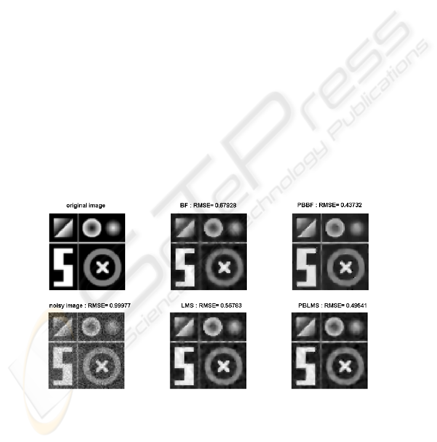
The results of the denoising procedures are shown in Table 1. The PBBF outper-

forms both the classical BF and LMS approaches in terms of RMSE and visual ap-

preciation (see Fig. 2). The mechanisms behind theses performances can be explained:

optimal parameters for this ﬁlter use narrow radiometric (small σ in equation 6) and

spatial kernels (small ρ in equation 4), but a larger (13) number of iterations, whereas

the BF usually converges to a constant solution after more than 3 iterations.

As the PBBF is more selective than the BF for the computation of the weights, it can

use a higher number of iterations and narrow radiometric and spatial kernels to converge

slowly toward a better ﬁltering result. The PBBF outperforms the other algorithms on

all parts of the image.

The reason why the PBLMS is less performant than the PBBF can be explained too.

After the ﬁrst iteration, the algorithm computes the distance between the last estimated

image P

and the observed image P

. As the ﬁltering effect is applied on the estimated

Fig. 2. Top row: left, original image. Middle, bilateral ﬁltered image. Right, patch-based ﬁltered

image. Bottom row: left, noisy image. Middle, local M-smoother ﬁltered image. Right, patch-

based local M-smoother ﬁltered image.

image, those images get more and more different, and the differences add up in the

distance computation until the distance is large enough to eventually be out of the ra-

diometric kernel range and thus reduces the weight to almost zero. The ﬁltering process

is then stopped too early and the image is not ﬁltered anymore after a few iterations.

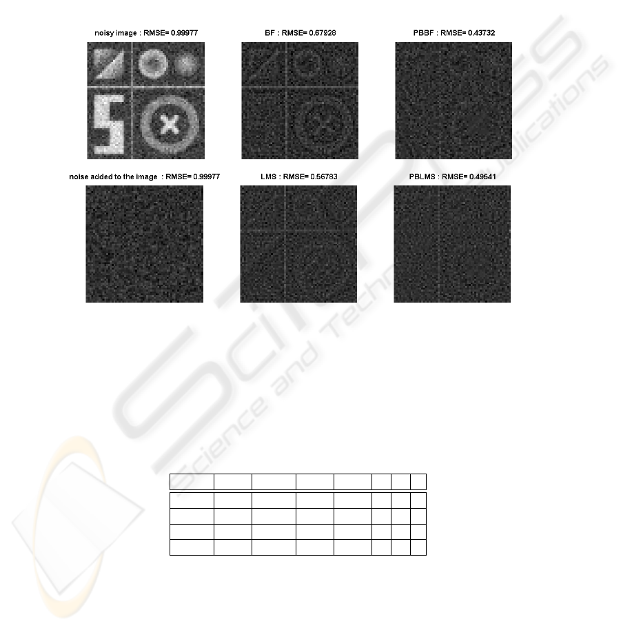
Fig. 3 shows the residuals of the ﬁltered images. The residuals for the PBBF and

PBLMS ﬁltered image have almost no structure while the BF and LMS ones contain

parts of the original image, it shows that in theses cases, the ﬁltering effect was not

optimal.

Fig. 3. Top row: left, noisy image. Middle, residuals of the bilateral ﬁltered image. Right, residuals

of the patch-based bilateral ﬁltered image. Bottom row: left, noise added to the original image.

Middle, residuals of the local M-smoother ﬁltered image. Right, residuals of the patch-based local

M-smoother ﬁltered image.

Table 1. Mean RMSE over the 100 test images for the different algorithms and masks (2D). ρ, σ

and n are respectively the width of the spatial kernel, radiometric kernel, and number of iterations

of the ﬁlter.

image plateaus edges ramps ρ σ n

PBBF 0.4373 0.2637 0.5941 0.5484 2.1 0.3 15

PBLMS 0.4954 0.3866 0.6272 0.4995 2.8 0.6 5

BF 0.5614 0.4033 0.7464 0.5695 1.9 2.6 2

LMS 0.5678 0.4051 0.7565 0.5491 2.5 2.6 3

These algorithms were tested on 3D images. In this case we generated 100 images

of dimension 64 ×64 × 100 with the same noise model, and used p × p × p patches and

3D kernels. The RMSE is calculated over each one of these 64 × 64 × 100 images for

all algorithms. In the 3D case, the performances of all algorithms improve (see Table

2). The PBBF ﬁltering algorithm still gives the best RMSE, on all areas of the image.

Obviously, the benchmark image that was used here is constituted of the same slices

which help the denoising algorithms a lot. However, successive slices are usually highly

correlated in real 3D images, therefore the PBBF may ﬁnd some useful informations

when a third dimension is added. Further experiments should be done on 3D benchmark

images in order to conﬁrm the ﬁltering gain that we noticed on the 3D denoising.

Table 2. mean RMSE over the 100 test images for the different algorithms and masks (3D). ρ, σ

and n are respectively the width of the spatial kernel, radiometric kernel, and number of iterations

of the ﬁlter.

image plateaus edges ramps ρ σ n

PBBF 0.2515 0.1432 0.3348 0.3941 2.1 0.3 13

PBLMS 0.3493 0.2380 0.4721 0.3765 2.8 0.6 5

BF 0.4045 0.2982 0.5290 0.4281 2.1 1.8 2

LMS 0.4228 0.3294 0.5366 0.4387 2.2 2 3

The PBBF algorithm was also compared to the BF on a phantom CT image. A

phantom consists of several cylinders of different densities. As the absorption properties

of the cylinders are known, the images acquired on these phantoms a used to determine

the quantity and distribution of the noise generated in the acquisition process. This

time, the parameters of the ﬁlters were ﬁxed empirically as they would have been for a

classical CT image for which no ground truth is available. The quality of the denoising

effect was evaluated from the residuals: the difference between the original and the

denoised image. Figure 4 shows the PBBF and BF denoised images ans their residuals.

From visual evaluation, they seem very close in quality: for both algorithms, there is

no visible blurring induced in the denoising process and the residual noise is located at

the same areas. Still, the residuals from the PBBF algorithm show slightly less structure

than those from the BF algorithm, which shows that the PBBF preserved the edges in a

more efﬁcient way. The PBBF seems to at least compare to the BF on images acquired

with real scanners. More experiments on real medical images will be done in the future.

4 Conclusions

In this paper, we introduced the patch-based bilateral ﬁlter and patch-based local M-

smoother. The introduction of patches in the classical bilateral ﬁlter and local M -

smoother algorithms is based on the idea that an algorithm using more than one voxel

at a time might be able to be more sensitive to the textures and ramps of the image.

Our experiments shows that the patch-based bilateral ﬁlter outperforms the bilateral ﬁl-

ter and local M-smoother algorithms both in terms of RMSE and visual appreciation.

These results also seems promising in the 3D denoising tasks. In the future, we will

adapt this method to more complex noise models (i.e. Poisson or multiplicative noise)

and other patch-to-patch distances functions will be implemented and tested. More per-

formances evaluations of these algorithms will be done on CT-scan or PET-scan images

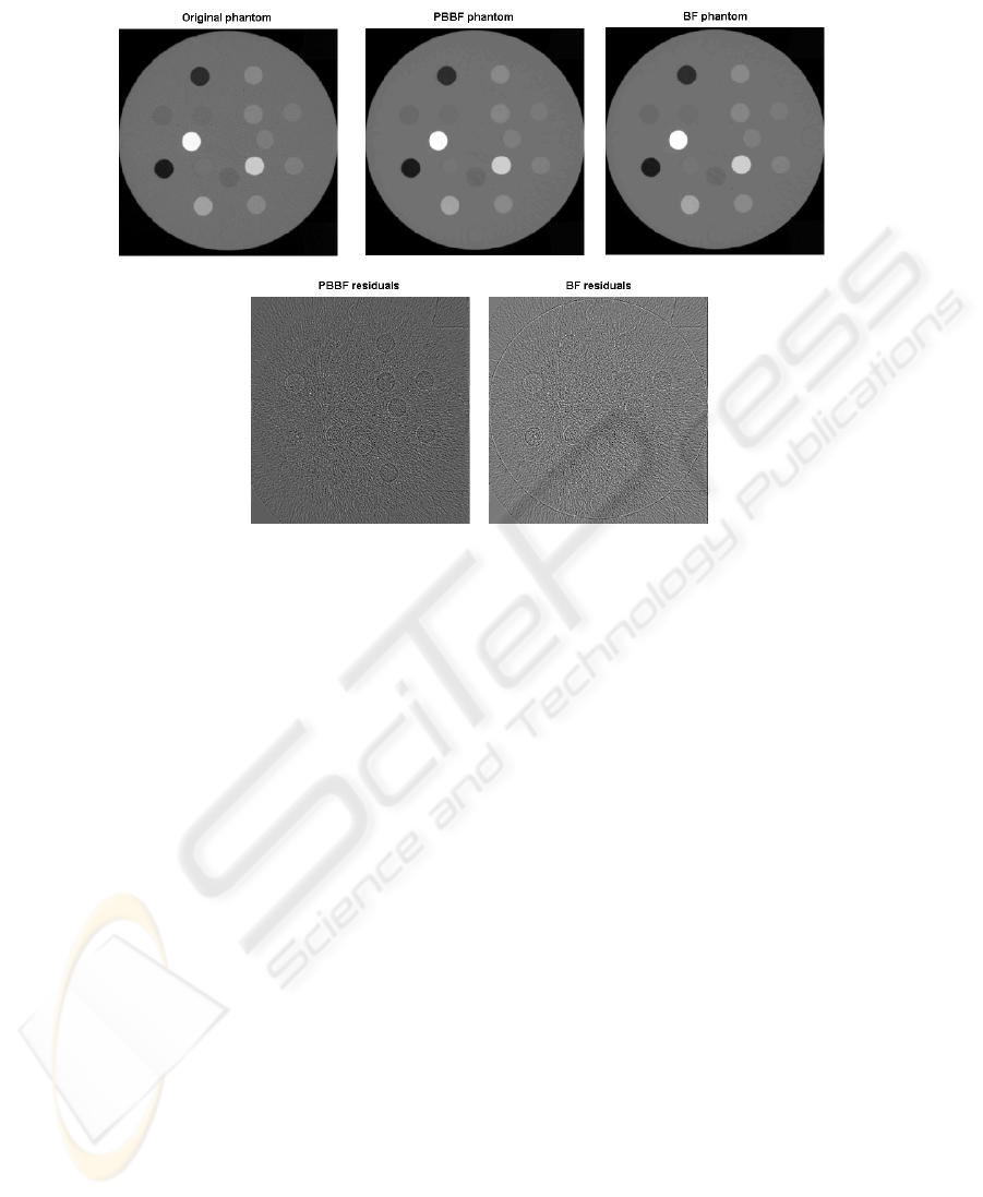
Fig. 4. Top row: left, original phantom image. Middle, PBBF denoised phantom. Right, LMS

denoised image. Bottow row: left, residuals for the PBBF image. Right residuals for the BF

denoised image.

and the results will be assessed by oncologists within the framework of tumor and organ

delineation tasks.

Acknowledgements

A. de Decker is funded by a Belgian F.R.I.A. grant. J.A. Lee is a Postdoctoral Re-

searcher funded by the Belgian National Fund of Scientiﬁc Research (FNRS).

References

1. Charnigo, R., Sun, J., Muzic, R.: A semi-local paradigm for wavelet denoising. IEEE Trans

Image Process 15 (2006) 666–677

2. Lin, J.W., Laine, A.F., Bergmann, S.R.: Improving pet-based physiological quantiﬁcation

through methods of wavelet denoising. IEEE Trans Biomed Eng 48 (2001) 202–212

3. Bruni, V., Piccoliand, B., Vitulano, D.: Wavelets and partial differential equations for image

denoising. Electronic Letters on Computer Vision and Image Analysis 6 (2008) 36–53

4. Osher, S., Burger, M., Donald, G., Jinjun, X., Yin, W.: An iterative regularization method

for total variation-based image restoration. Multiscale Model. Simul. 4 (2005) 460–489

5. Sanches, J.M., Nascimento, J.C., Marques, J.S.: An uniﬁed framework for bayesian denois-

ing for several medical and biological imaging modalities. Conf Proc IEEE Eng Med Biol

Soc 1 (2007) 6267–6270

6. Takeda, H., Farsiu, S., Milanfar, P.: Kernel regression for image processing and reconstruc-

tion. IEEE Transactions on Image Processing 16 (2007) 349–365

7. Huang, R.H., Wang, X.H.: Image denoising via gradient approximation by upwind scheme.

Signal Processing, 88 (2008) 69–74

8. Mrazek, P., Weickert, J., A., B.: On Robust Estimation and smoothing with Spatial and Tonal

Kernels. In: Geometric Properties for Incomplete data. (2006) 335–352

9. Chu, C., Glad, I., Godtliebsen, F., J.S., M.: Edge-preserving smoothers for image processing.

Journal of the American Statistical Association, 93,no.442 (1998) 526556

10. Elad, M.: On the origin of the bilateral ﬂter and ways to improve it. IEEE Trans. Image

Processing, 11 (2002) 11411151

11. Tomasi, C., Manduchi, R.: Bilateral ltering for gray and color images. In: 6th Int. Conf.

Computer Vision, pp.839846. (1998)

12. Wong, W., Chung, A., Yu, S.: Trilateral ﬁltering for biomedical images. In Chung, A.,

ed.: Proc. IEEE International Symposium on Biomedical Imaging: Nano to Macro. (2004)

820–823 Vol. 1

13. Kervrann, C., Trubuil, A.: An adaptive window approach for poisson noise reduction and

structure preserving in confocal microscopy. In Trubuil, A., ed.: Proc. IEEE International

Symposium on Biomedical Imaging: Nano to Macro. (2004) 788–791 Vol. 1

14. Kervrann, C., Boulanger, J.: Optimal spatial adaptation for patch-based image denoising. ,

15 (2006) 2866–2878

15. Lee, J., Geets, X., Gregoire, V., Bol, A.: Edge-preserving ﬁltering of images with low photon

counts. IEEE Transactions on pattern analysis and machine intelligence, 30 (2008) 1014–

1027