EAR SEGMETATION USING TOPOGRAPHIC LABELS

Milad Lankarany and Alireza Ahmadyfard

Department of Electrical Engineering and Robotics, Shahrood University of Technology, Shahrood, Iran

Keywords: Ear Biometrics, Ear Segmentation, Topographic Features.

Abstract: Ear segmentation is considered as the first step of all ear biometrics systems while the objective in

separating the ear from its surrounding backgrounds is to improve the capability of automatic systems used

for ear recognition. To meet this objective in the context of ear biometrics a new automatic algorithm based

on topographic labels is presented here. The proposed algorithm contains four stages. First we extract

topographic labels from the ear image. Then using the map of regions for three topographic labels namely,

ridge, convex hill and convex saddle hill we build a composed set of labels. The thresholding on this

labelled image provides a connected component with the maximum number of pixels which represents the

outer boundary of the ear. As well as addressing faster implementation and brightness insensitivity, the

technique is also validated by performing completely successful ear segmentation tested on “USTB”

database which contains 308 profile view images of the ear and its surrounding backgrounds.

1 INTRODUCTION

Ear images can be acquired in a similar manner to

face images and a number of researchers have

suggested that the human ear is unique enough to

each individual to allow practical use as a biometric.

Bhanu and Chen (2003) presented a 3D ear

recognition method using a local surface shape

descriptor. Twenty range images from 10 individuals

are used in the experiments and a 100 percent

recognition rate is reported. Chen and Bhanu (2005)

used a two-step ICP algorithm on a data set of 30

subjects with 3D ear images. They reported that this

method yielded two incorrect matches out of 30

people. In these two works, the ears are manually

extracted from profile images. They also presented

an ear detection method in (Bhanu, 2004). In the

offline step, they built an ear model template from

each of 20 subjects using the average histogram of

the shape index. In the online step, first, they used

step edge detection and thresholding to find the

sharp edge around the ear boundary and then applied

dilation on the edge image and connected

component labelling to search for ear region

candidates. Each potential ear region is a rectangular

box, and it grows in four directions to find the

minimum distance to the model template. The region

with minimum distance to the model template is the

ear region. They get 91.5 percent correct detection

with a 2.5 percent false alarm rate. No recognition

results are reported based on this detection method.

Hurley et al developed a novel feature extraction

technique using force field transformation. Each

image is represented by a compact characteristic

vector which is invariant to initialization, scale,

rotation, and noise. The experiment displays the

robustness of the technique to extract the 2D ear.

The data set comes from the XM2VTS face image

database. Choras introduces an ear recognition

method based on geometric feature extraction from

2D images of the ear. The geometric features are

computed from the edge detected intensity image.

They claim that error-free recognition is obtained on

“easy” images from their database. The “easy”

images are images of high quality with no earring

and hair covering and without illumination changes.

No detailed experimental setup is reported.

There are a number of algorithms based on force

field transforms to deal with segmentation. Luo et al

describe the use of Vector Potential to extract

corners by treating the “Canny” edge map of an

image as a current density. Ahuja used a novel force

field segmentation technique where pixels of similar

intensity were detected by assigning inter-pixel

forces inversely proportional to the grey level

difference. Ahuja and Chuang used a potential field

model to extend the medial axis transform. Xu and

Prince extended the active contour model by

186

Lankarany M. and Ahmadyfard A. (2009).

EAR SEGMETATION USING TOPOGRAPHIC LABELS.

In Proceedings of the Fourth International Conference on Computer Vision Theory and Applications, pages 186-191

DOI: 10.5220/0001797601860191

 SciTePress

replacing the external local force with a force field

derived from the image edge map.

Yan et al present the first fully automated system

for ear biometrics using 3D shape. There are two

major parts of the system: automatic ear region

segmentation and 3D ear shape matching. Starting

with the multimodal 3D + 2D image acquired in a

profile view, the system automatically finds the ear

pit by using skin detection, curvature estimation, and

surface segmentation and classification. After the ear

pit is detected, an active contour algorithm using

both colour and depth information is applied to

outline the visible ear region.

Except the Yan's method that automatically

approached ear-segmentation using 3-D information

of the profile images, the works based on edge

detection algorithms present automated approaches

for ear-segmentation using only 2-D images of the

ear. In this case, the edge image of the ear and

surroundings is first obtained then distinctive

contours are recognized. It is experimentally

concluded that the contour which includes the

maximum number of pixels, points out to the edge

of outer ear. Therefore the ear boundary can be

found easily according to that contour. However,

this technique suffers two main problems. First

problem is caused by the dependence of edge

detection algorithms to thresholding value. Second

one arises from the discontinuity of contours

obtained from the edge detector. In some cases,

several pixels of a same contour, which is detectable

using human’s eyes, are disconnected therefore; the

separated contours are recognized wrongly. This

effect is illustrated in figure 1.

(a) (b) (c)

Figure 1: (a). A profile image from USTB database, (b).

The edge image using “canny” operator with threshold 0.2

(c). The edge image with threshold 0.1 (the red line and

ellipse show the discontinuity of contours).

These problems motivated us to use a method

leading to obtain more reliable regions (instead of

edge contours) free from threshold selection.

Providing this purpose, we used topographic map of

ear image and label it. Each pixel in ear image is

described by one of the twelve topographic labels.

No predefined threshold is needed to label the image

in this manner. On the other hand, more geometric

properties of the ear image are yielded. Three labels,

namely, ridge, convex hill and convex saddle hill

which are selected experimentally, are combined in

order to extract the ear outline. More consideration

in outer ear shape shows that this part of ear is fully

described by the convex hill and convex saddle hill

labels. Moreover the ridge label in the ear image is

similar to the image edges, but the extraction of the

ridge label is independent of threshold value. Figure

2 shows the each of those labels extracted from a

test ear. It is experimentally concluded that the

connected component obtained from the

combination of topographic labels consisting of the

maximum number of pixels matches to the image of

outer ear. As a result the boundary of this region

demonstrates the ear in an ear image.

(A) (B) (C) (D)

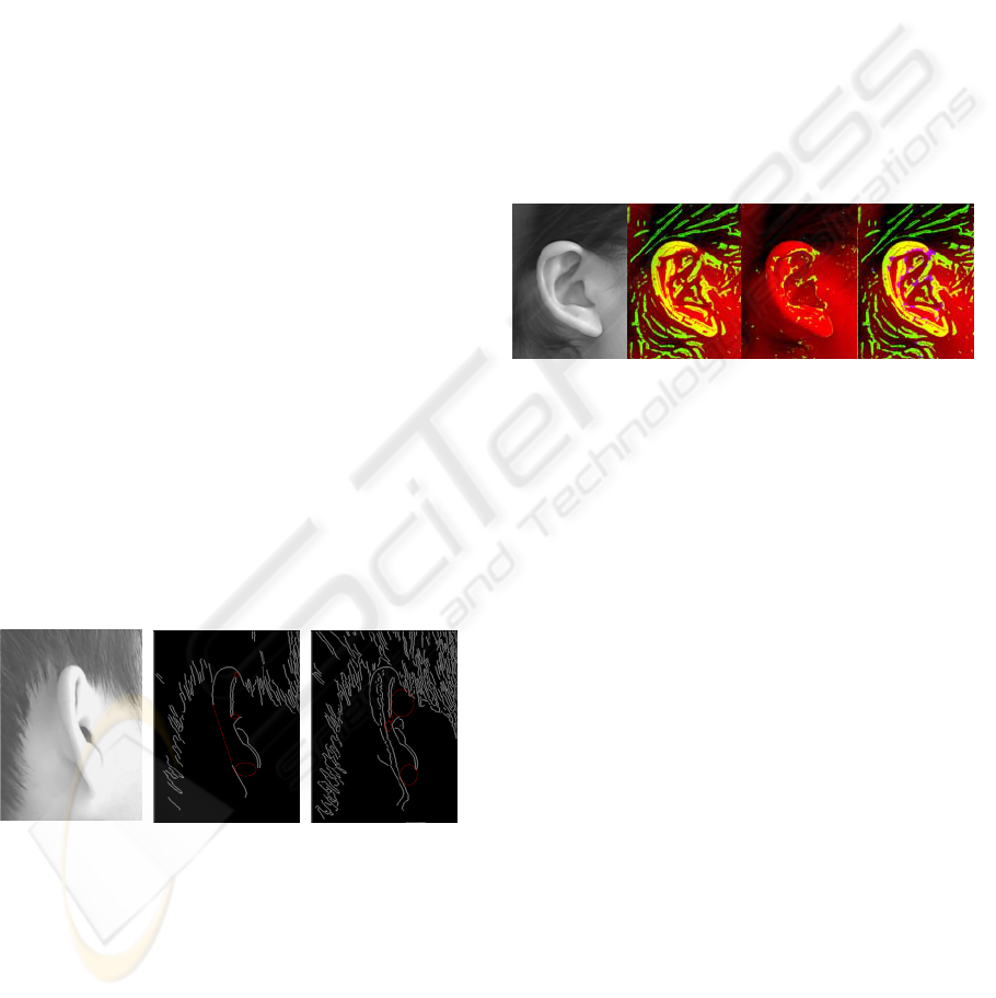
Figure 2: (A). Selected image from USTB database, (B).

Green part shows the convex hill label, (C). Green part

indicates the convex sadlle hill, (D). Green part shows

convex hill and blue part shows the convex saddle hill

label, all extracted from selected ear image.

2 TOPOGRAPHIC LABELS

Using topographic models for representing images

has been reported in computer vision literature

((M.Haralick, 1983), (J.Wang, 2007)). This method

is classified in appearance based category. The main

advantage of using topographic features for

representation respect to intensity is its robustness to

lighting condition (L.Wang, 1993).

Consider a grey scale ear image as a surface in 3D

space where x and y axes are along image

dimensions. The value of surface at pixel (x,y) is the

pixel intensity f(x,y). Depending on the topographic

property of surface at each pixel one of twelve

topographic labels in Figure 3 is assigned to the each

pixel. In order to label intensity image based on

topographic property let us consider the input image

as a continues function f(x,y). The topographic label

at each pixel of image is determined using first and

second order derivatives on surface f.

EAR SEGMETATION USING TOPOGRAPHIC LABELS

187

Considering the Hessian matrix of this function as

follows:

(1) (1)

After applying eignvalue decomposition to the

Hessian matrix we have:

12 12 12

[].().[... ... ]

HUDU

uudiag uu

λλ

(2)

Where

,uu

point out to the eigenvectors of H and

λλ

are the eigenvalues of the Hessian matrix.

Also

ff ∇∇

correspond to the derivative vector

of function

(the surface intensity) and its

magnitude, respectively, should be computed.

(,) (,)fxy fxy

⎛⎞

∂∂

∇= −

⎜⎟

∂∂

⎝⎠

(3)

(4)

Figure 3: Topographic labels (a) peak (b) pit (c) ridge (d)

ravine (e) ridge saddle (f) ravine saddle (g) convex hill (h)

concave hill (i) convex saddle hill (j) concave saddle hill

(k) slop hill and (l) flat.

In this part we only consider the labels used in this

paper. These labels are ridge, convex hill, convex

saddle hill. For further details on determining other

topographic labels one can refer to (L.Wang, 1993).

It is worth to note that image noise can cause an

undesired result of topographic labelling. As shown

by Wang et al (1993) a smoothing filter before

topographic labelling provide more acceptable

result. For this purpose we filter input image using a

Gaussian kernel before the labelling. The filter

parameters should be selected based on the size of

interest pattern (ear) and the level of input noise.

Ridge: this label assigns to pixel (x,y) if one of the

following criteria is satisfied.

(5) (5)

Convex hill: this label assigns to pixel (x,y) if one of

the following criteria is satisfied.

(6)

Convex saddle hill: this label assigns to pixel (x,y)

if the following criterion is satisfied.

(7)

Figure 4 (up) is plotted to indicate 3 mentioned

labels extracted of figure 2.A.

3 EAR SEGMENTATION

A. Label Extraction: according to last section, 3

labels, namely, ridge, convex hill and convex saddle

hill are extracted from each profile image. Figure 4

(down) shows the combination of these labels.

B. Thresholding: the image approached by

combining those three labels is binary (intensities

are “0” or “1”). The pixels whose intensities are “1”

are replaced by their original intensity values from

the profile image. These values are scaled in the

range of grey level (“0” to “255”). The achieved

image is enhanced by using histogram equalization.

At last by defining threshold value as “150” (in grey

level) the pixels whose intensity values are lower

than that threshold are mapped to “0” and the other

pixels give “1” as their intensity value. Figure 5

demonstrates the image yielded by using this step. It

should be noted that this step is not an essential part

of our algorithm and the proposed algorithm

operates accurately without using this step. But a

considerable reduction in computation complexity is

achieved by using this step. As compared with figure

4 (down), the excessive contours around the ear can

be easily omitted using this step.

C. Finding the Region of Outer Ear: as mentioned

in introduction, it is experimentally concluded that

the contour which contains the maximum number of

pixels covers the region of the outer ear. Figure 6

shows this contour which is extracted of figure 5.

For this purpose (finding the contours of a binary

image) we use “bwlabel” a command of MATLAB.

VISAPP 2009 - International Conference on Computer Vision Theory and Applications

188

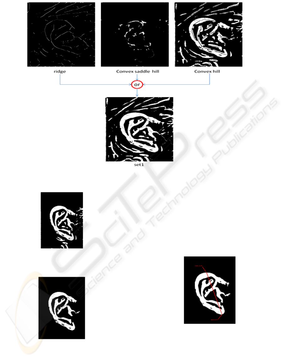
Figure 4: Up. Three topographic labels obtained for profile image shown in figure 2.A Down. The combination of those

labels.

Figure 5: The combination of three mentioned topographic

labels after thresholding.

Figure 6: the contour includes the maximum number of

pixels.

D. Two Landmark Points: because the features for

a recognition algorithm should be invariant to

translation and scale change, the normalization step

is performed. The normalization process is done

with respect to scale and rotation. This is done by

finding a two point land mark (figure 7) in every

contour approached in step C. These two points can

be easily determined by finding the pixels assigned

to maximum and minimum values of coordinate axis

in the vertical direction.

Figure 7: Two landmark points, which correspond to

maximum and minimum values of vertical axis, are

identified in the contour approached in step C followed by

dilating.

E. Scaling and Rotation: After detecting those

points, the profile image is transformed with respect

to those landmarks to a new location. This

transformation will result in getting the landmark

EAR SEGMETATION USING TOPOGRAPHIC LABELS

189

points in all images to have the same distance

between them and that orientation of the line

connecting the two landmark points will be vertical

in the image. Figure 8 demonstrates the result of this

normalization applied to profile image shown in

figure 2.A.

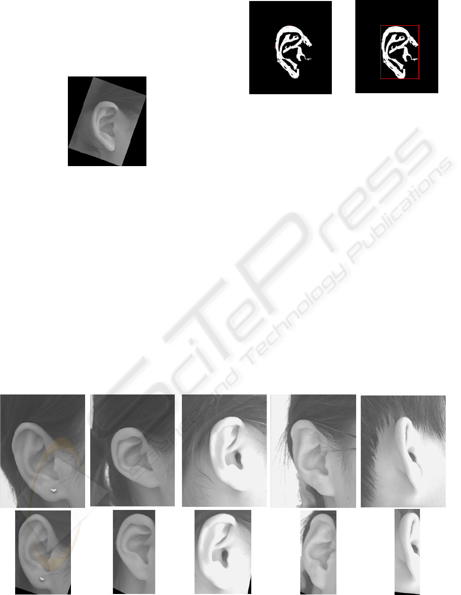
Figure 8: The result of normalization of profile image with

respect to rotation.

F. Foure Landmark Points: step E (normalization)

is first applied to the contour yielded in step C then,

a 4 point landmark, which are shown in figure 9.A,

are selected by finding the maximum and minimum

values of coordinate axises in both vertical and

horizontal directions. A rectangular window

separates the region of normalized ear from it’s

surroundings based on points obtained in step F.

Figure 9.B shows this window.

At last by applying this window to the

normalized profile image approached in step E, the

segmented ear will be obtained.

(A) (B)

Figure 9: (A). Four land mark points founded in the

normalized contour which approached by applying step E

to the contour obtained in step C, (B). The window which

is drawn based on the landmark points.

3.1 Segmentation Results

Our algorithm achieves fully successful ear

segmentation on USTB database which includes 77

subject dataset, 4 images for each subject. Some

profile images selected of our used database are

shown in figure 10.A. Ear segmentation based on

proposed algorithm achieves 100 percent true

segmentation while applying edge detection

algorithm according to “Canny” method, yielded

67.2 percent true segmentation. Both methods are

tested on the USTB database. Wrong segmentation

corresponds to incomplete separation of ear from

surroundings. Figure 10.B demonstrates some

segmented ears, which are separated from profile

images shown in figure 10.A, approached by our

proposed algorithm.

Figure 10: A. Some samples from ear images in USTB database (first row), B. The results of segmentation of the first row

using the proposed algorithm (second row).

VISAPP 2009 - International Conference on Computer Vision Theory and Applications

190

4 CONCLUSIONS

We have presented an automatic ear segmentation

approach using 2D images. The automatic ear

extraction algorithm can separate the ear from

surrounding area including hair. The proposed

method uses topographic labels to obtain a reliable

region representing outer ear. The experimental

results demonstrate the power of our automatic ear

extraction algorithm when it is compared with edge

detection based techniques. The proposed system

successfully segments all ear images in USTB

database.

REFERENCES

Ping Yan and Kevin W.Bowyer “Biometric Recognition

Using 3-D Ear Shape”, IEEE Trans. PAMI, VOL. 29,

NO. 8, 2007

David J. Hurley, Mark S. Nixon, John N. Carter “Force

Field Feature Extraction for Ear Biometrics”,

Computer Vision and Image Understanding

ELSEVIER.

B. Bhanu and H. Chen, “Human Ear Recognition in 3D,”

Proc.Workshop Multimodal User Authentication, pp.

91-98, 2003.

D. Hurley, M. Nixon, and J. Carter, “Force Field Energy

Functionals for Image Feature Extraction,” Image and

Vision Computing J., vol. 20, pp. 429-432, 2002.

H. Chen and B. Bhanu, “Human Ear Detection from Side

Face Range Images,” Proc. Int’l Conf. Image

Processing, pp. 574-577, 2004.

H. Chen and B. Bhanu, “Contour Matching for 3D Ear

Recognition,” Proc. Seventh IEEE Workshop

Application of Computer Vision,pp. 123-128, 2005.

K. Messer, J. Matas, J. Kittler, J. Luettin, and G. Maitre,

“XM2VTSDB: The Extended M2VTS

Database,”Audio and Video-Based Biometric Person

Authentication, pp. 72-77, 1999.

M. Choras, “Ear Biometrics Based on Geometrical Feature

Extraction,” Electronic Letters on Computer Vision

and Image Analysis, vol. 5, pp. 84-95, 2005.

M. Choras, “Further Developments in Geometrical

Algorithms for Ear Biometrics,” Proc. Fourth Int’l

Conf. Articulated Motion and Deformable Objects, pp.

58-67, 2006.

B. Luo, A.D. Cross, E.R. Hancock, “Corner detection via

topographic analysis of vector potential”, Pattern

Recognition Letter. 20 (6) (1999) 635–650.

N. Ahuja, “A transform for multiscale image segmentation

by integrated edge and region detection”, IEEE Trans.

PAMI 18 (12) (1996) 1211–1235.

N. Ahuja, J.H. Chuang, Shape representation using a

generalized potential field model, IEEE Trans. PAMI

19 (2) (1997) 169–176.

Li Yuan, Zhichun Mu, Zhengguang Xu, “Using Ear

Biometrics for Personal Recognition”, IWBRS 2005,

Beijing, China, October 2005, 221-228.

C. Xu, J.L. Prince, “Gradient vector flow: a new external

force for snakes”, in: Proc. IEEE Conf. on Computer

Vision and Pattern Recognition (CVPR), 1997, pp.

66–71.

R. M. Haralick. L. T. Watson, and T. J. Laffey, "The

topographic primal sketch," Int. J . Robotics Res. vol.

2, pp. 50-72, 1983.

J. Wang, and L. Yin, "Static topographic modeling for

facial expression recognition and analysis," Computer

Vision and Image Understanding Journal, vol. 108, pp.

19-34, October 2007.

L. Wang, and T. Pavlidis."Direct Gray-Scale Extraction of

Features for Character Recognition",IEEE Trans.

PAMI. vol. 15, no. 10, pp.1053-1067, October 1993.

EAR SEGMETATION USING TOPOGRAPHIC LABELS

191