ASSIGNING AUTOMATIC REGULARIZATION PARAMETERS IN

IMAGE RESTORATION

Ignazio Gallo and Elisabetta Binaghi

Universit

a degli Studi dell’Insubria, via Ravasi 2, Varese, Italy

Keywords:

Regularization proﬁle, Image restoration, Adaptive regularization, Neural networks.

Abstract:

This work aims to deﬁne and experimentally evaluate an adaptive strategy based on neural learning to select

an appropriate regularization parameter within a regularized restoration process. The appropriate setting of

the regularization parameter within the restoration process is a difﬁcult task attempting to achieve an optimal

balance between removing edge ringing effects and suppressing additive noise. In this context,in an attempt to

overcome the limitations of trial and error and curve ﬁtting procedures we propose the construction of the reg-

ularization parameter function through a training concept using a Multilayer Perceptron neural network. The

proposed solution is conceived independent from a speciﬁc restoration algorithm and can be included within

a general local restoration procedure. The proposed algorithm was experimentally evaluated and compared

using test images with different levels of degradation. Results obtained proven the generalization capability of

the method that can be applied successfully on heterogeneous images never seen during training.

1 INTRODUCTION

Restoration of blurred and noisy images requires the

adoption of a regularization approach based on the

speciﬁcation of a cost function consisting of a least

square term and a regularization term (Lagendijk and

Biemond, 2001; Andrews and Hunt, 1977). The role

of the two terms is controlled by the regularization pa-

rameter. The appropriate setting of the regularization

parameter within the restoration process achieves an

optimal balance between removing edge ringing ef-

fects and suppressing additive noise.

The critical problem of optimally estimating the

regularization parameter has been investigated in

depth in literature.

Previous works addressed the problem by propos-

ing a regularization proﬁle where the local parame-

ter value is expressed as a monotonically decreasing

function of the local variance (Qian and Clarke, 1996;

Lagendijk et al., 1988; Katsaggelos and Kang, 1995).

In particular Perry and Guang (Perry and Guan, 2000)

proposed a perceptually motivated solution in which

the constraint values decrease linearly as the loga-

rithm of the local regional variance increases. Pro-

ceeding from these results, in a previous work we de-

ﬁned a statistics-based procedure assigning a separate

parameter to each image pixel according to local vari-

ance computed in the neighborhood of the pixel to be

examined.

The regularization parameter is speciﬁed for each

pixel as λ(x, y) = Y (S(x, y)) where S(x, y) is the lo-

cal variance of the degraded input image g varying

from S

min

to S

max

, while Y corresponds to the log-

linear function:

Y (S; λ

min

, λ

max

) = (1)

min

− λ

max

− S

min

(log(S) − S

min

) + λ

max

To determine the function Y univocally and then build

a speciﬁc regularization proﬁle, we need to ﬁx values

min

and λ

max

corresponding to S

max

and S

min

respec-

tively.

The present work proposes a novel approach to

regularization proﬁle estimation based on the approx-

imation capability of the supervised neural learning

technique based on Multilayer Perceptron Network

(MLP). The interest in this novel strategy mainly lies

in the possibility of inducing the regularization func-

tion from a set of training images, directly mapping

local variance values and/or other image features to

regularization parameters without requiring trial and

error and curve ﬁtting procedures.

Gallo I. and Binaghi E. (2009).

ASSIGNING AUTOMATIC REGULARIZATION PARAMETERS IN IMAGE RESTORATION.

In Proceedings of the Fourth International Conference on Computer Vision Theory and Applications, pages 74-77

DOI: 10.5220/0001785500740077

 SciTePress

2 THE PROPOSED METHOD

The proposed method for regularization parameter

assignment is conceived as a pre-processing phase

within a general restoration strategy. To make the pa-

per self-contained and to exploit all the ingredients of

the overall strategy adopted in the experimental part

of the work, we brieﬂy outline the salient aspects of a

restoration strategy developed and presented in a pre-

vious study. It consists of a neural iterative method

which uses a gradient descent algorithm to minimize

a local cost function derived from a traditional global

constrained least square measure (Gallo et al., 2008).

In particular, the degradation measure to be min-

imized is a local cost function E(x, y) deﬁned at any

point (x, y) in an M × N image:

E(x, y) =



g(x, y) − h ∗

f (x, y)



+ (2)

λ(x, y)



d ∗

f (x, y)



where h ∗

f (x, y) denotes the convolution between a

blur ﬁlter h centered in a point (x, y) of the restored

image

f and the restored image

f itself; d ∗

f (x, y)

denotes the convolution between a high-pass ﬁlter d

centered in a point (x, y) of the restored image

f and

the restored image

f itself.

A multilayer perceptron model, trained with

the supervised back propagation learning algo-

rithm (Rumelhart et al., 1986), was adopted to com-

pute the regularization parameter based on speciﬁc

local information extracted from the degraded image

g(x, y) previously scaled in a range [0, 1]. The neural

learning task accomplished within the neural training

phase can be formulated as a search for the best ap-

proximation of the function λ(x, y) =Y (S

) where S

represents a set of statistical measures extracted di-

rectly from the degraded image. The present work

uses S

= (S

(x, y), S

) where S

is the lo-

cal variance computed directly on the degraded im-

age and S

is the local variance computed on the de-

graded image smoothed with a Gaussian low-pass ﬁl-

ter. In particular we use the variance calculated in a

window measuring 3 × 3 as statistical measure S

and

the variance calculated in a window measuring 5 × 5

as statistical measure S

The joint use of S

and S

is motivated by the need

to preserve image features during restoration. S

is a

constant value derived from the histogram of S

. In

particular S

is the value of variance corresponding to

the peak value in the histogram. This is an important

feature because it is directly correlated to the amount

of noise in the degraded image and we know that λ

should be proportional to the amount of noise in the

data (Inoue et al., 2003).

The training set presented to the neural network

for the supervised learning task is constituted by

N pairs of elements ((S

, S

)

where n =

1, . . . , N. The second component of training examples

are the expected outputs for the corresponding in-

put components and are constituted by regularization

values obtained from successful restoration processes

as explained in section 2.1.

The trained network is expected to be able to gen-

eralise, i.e. to associate adequate regularization val-

ues with degraded input images never seen during

training.

2.1 Regularization Proﬁle Construction

Representative samples of the function λ(x, y) =

Y (S

) are necessary if we want to train a neural net-

work that represents it. Algorithm 1 describes in de-

tails the method used to compute a sampling of this

function while Figure 1 shows an example of tabular

data obtained from the same algorithm. Representa-

tive samples of the function λ(x, y) = Y (S

) must be

presented to the network during the training phase for

learning. Algorithm 1 describes the procedure used to

build the sample pairs ((S

, S

)

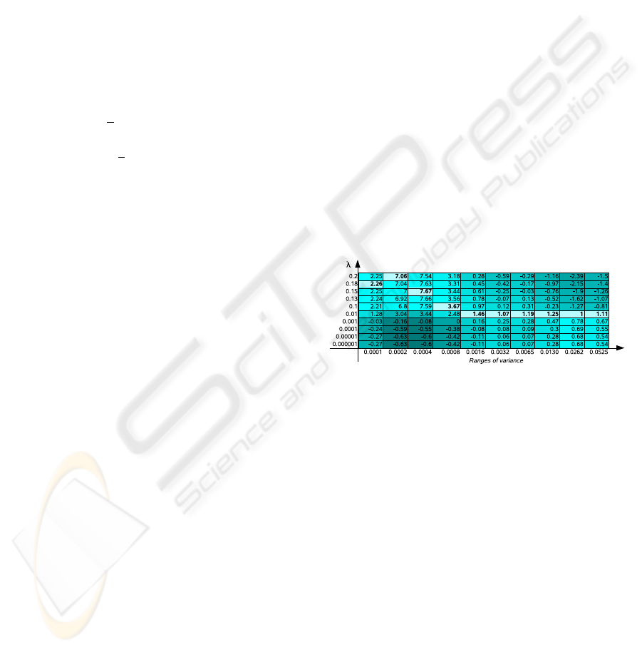
Figure 1: The columns list the ISNR values obtained restor-

ing the image with a set of different constant λ values. Each

column identiﬁes a group of pixels with variance included

in a preﬁxed range. The best λ value for a given range of

variance corresponds to the highest ISNR values obtained

(in bold) .

Our approach compares the improvement in sig-

nal to noise ratio (ISNR) measures calculated on a set

of restored pixels

f (x, y), all having a statistical mea-

sure included in an interval I

≤ S(x, y) < I

i+1

. Then

we choose the best

λ corresponding to the best ISNR.

The result of this approach is an approximation of the

function λ(x, y) = Y (S

) representing the regulariza-

tion proﬁle with which to compute the regularization

parameter.

The training set is built applying Algorithm 1 to a

set of images representative of a given domain. To be

exhaustive, each image in turn must be degraded with

different levels of noise and different kinds of blur.

ASSIGNING AUTOMATIC REGULARIZATION PARAMETERS IN IMAGE RESTORATION

Algorithm 1 - function λ(x, y) = Y (S

) sampling.

Require: to select a degraded image g(x, y) and the

corresponding undistorted image f (x, y);

Require: to break in R regular intervals I

, . . . , I

the

range [log(S

1,min

), log(S

1,max

)];

Require: to deﬁne a set of L regularization parame-

ters Λ = {λ

, . . . , λ

};

1: for j = 1 to L do

2: for s = 1 to R do

3: restore all the pixels belonging to the inter-

val I

using λ

as regularization parameter;

4: select the best parameter

, for all the pixels

belonging to the interval I

, choosing what

has maximized the ISNR measure;

5: end for

6: end for

7: Pattern set extraction

3 EXPERIMENTS

The proposed algorithm was experimentally evalu-

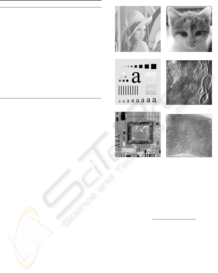
ated and compared using the six test images shown

in Figure 2. Images (a-c) were used to generate the

training set while images (d-f) were used as a test.

In the experiments all the test images were de-

graded by a Gaussian ﬁlter having standard deviation

= σ

= 1.0 and corrupted by Gaussian noise hav-

ing standard deviation σ = 5, 15, 25. During the train-

ing set construction, the blurred images (a-c) of Fig-

ure 2 without added noise, were also used.

Referring to Algorithm 1, the parameters used in

the experiments were:

• R = 15: the range of variance of each image used

in training was split into 15 intervals;

• for each interval, up to 300 patterns were selected;

• L = 15: the constant regularization param-

eters used in each interval Λ = {0.000001,

0.00001, 0.0001, 0.001, 0.01, 0.028, 0.046,

0.064, 0.082, 0.1, 0.12, 0.14, 0.16, 0.18, 0.2};

• the restoration algorithm was run for 20 iterations

for each different λ

applied to each range I

con-

sidered.

The input pattern was created by reading pixel val-

ues in a window 3× 3 centered on a particular pixel in

the two images S

(x, y) and S

(x, y). To these values

we added S

which is a constant value for each image.

In this way the network used has 19 input neurons, a

single output neuron and a hidden layer with 38 neu-

rons. The network was trained for 1000 epochs over

all the training examples.

(a) (b)

(e) (f)

Figure 2: Undistorted images used in training: Lena (a), Cat

(b), A (c); undistorted test images: Moon (d), Board (e) and

Fingerprint (f).

To evaluate the restoration performances of our

approach quantitatively, the well-known Improve-

ment in Signal-to-Noise Ratio (ISNR) measure (Ban-

hom and k. Katsaggelos, 1997) was adopted. This can

be estimated as follows:

ISNR = 10log

∑

x,y

( f (x, y) − g(x, y))

∑

x,y

( f (x, y) −

f (x, y))

(3)

where g(x, y) is the given degraded image and

f (x, y)

is the restored image. This measure can only be eval-

uated for controlled experiments in which the blur and

noise have been synthetically introduced. The maxi-

mally achievable ISNR depends strongly on the con-

tent of the image, the type of blur considered and the

signal-to-noise ratio of the blurred image.

Table 1 summarizes the ISNR values obtained

restoring all the images shown in Figure 2 with differ-

ent levels of degradation. The ISNR values are always

positive except for one case where the image to be re-

stored was corrupted by a smaller amount of noise.

However, comparing the ISNR values obtained with

VISAPP 2009 - International Conference on Computer Vision Theory and Applications

our algorithm (Table 1) and the ISNR values obtained

with the algorithm proposed in (Gallo et al., 2007)

and showed in Table 2, the results are very similar.

Table 1: ISNR measure obtained from the restoration of all

the pictures shown in Figure 2. The neural network was

trained for 1000 epochs on a subset of pixels extracted from

images Lena, A, and Cat. Finally the same network was

tested on images Moon, Fingerprint and Board.

Training Test

Image noise isnr Image noise isnr

Lena 5 2.05 Moon 5 0.42

Lena 15 7.35 Moon 15 4.16

Lena 25 9.40 Moon 25 6.45

A 5 0.24 Fingerpr. 5 -2.51

A 15 0.87 Fingerpr. 15 1.66

A 25 1.53 Fingerpr. 25 3.02

Cat 5 2.07 Board 5 1.72

Cat 15 7.19 Board 15 3.85

Cat 25 9.09 Board 25 5.41

Table 2: Best restoration results obtained by a different al-

gorithm using a trial and error approach.

Image noise (σ) λ

min

max

ISNR

Cat 5 0.000001 0.1 2.33

Cat 15 0.000001 0.2 7.31

Cat 25 0.15 0.2 9.13

4 CONCLUSIONS

As seen in our experimental context, the proposed

method for automatically assigning regularization pa-

rameters during restoration produces successful re-

sults and can be conceived as a general model for

adaptive regularization assignment within a restora-

tion procedures. The generalization capability of the

network used for estimating the regularization proﬁle

was proven using a different set of images for training

and test phases. Results obtained ensure that the solu-

tion proposed can be conceived for operational tools

addressing collections of heterogeneous images with-

out the need for retraining.

Future works will attempt to improve the feature

extraction/selection task to capture essential represen-

tative image features and investigate the generaliza-

tion capacity of the neural model in depth in relation

to different imagery.

REFERENCES

Andrews, H. C. and Hunt, B. R. (1977). Digital Image

Restoration. Prentice-Hall, New Jersey.

Banhom, M. R. and k. Katsaggelos, A. (1997). Digital im-

age restoration. IEEE Signal Processing Mag.

Gallo, I., Binaghi, E., and Macchi, A. (2007). Adaptive im-

age restoration using a local neural approach. In 2nd

International Conference on Computer Vision Theory

and Applications.

Gallo, I., Binaghi, E., and Raspanti, M. (2008). Semi-blind

image restoration using a local neural approach. In

Signal Processing, Pattern Recognition, and Applica-

tions, pages 227–231.

Inoue, K., Iiguni, Y., and Maeda, H. (2003). Image restora-

tion using the rbf network with variable regularization

parameters. Neurocomputing, 50:177–191.

Katsaggelos, A. K. and Kang, M. G. (1995). Spatially adap-

tive iterative algorithm for the restoration of astronom-

ical images. Int. J. Imaging Syst. Technol., 6:305–313.

Lagendijk, R. L. and Biemond, J. (2001). Iterative Identi-

ﬁcation and Restoration of Images. Springer-Verlag

New York, Inc., Secaucus, NJ, USA.

Lagendijk, R. L., Biemond, J., and Boekee, D. E. (1988).

Regularized iterative image restoration with ringing

reduction. Acoustics, Speech, and Signal Processing,

36(12):1874–1888.

Perry, S. W. and Guan, L. (2000). Weight assignment for

adaptive image restoration by neural networks. IEEE

Trans. on Neural Networks, 11:156–170.

Qian, W. and Clarke, L. P. (1996). Wavelet-based neural

network with fuzzy-logic adaptivity for nuclear image

restoration. In Proceedings of the IEEE, volume 84,

pages 1458–1473.

Rumelhart, H., Hinton, G. E., and Williams, R. J. (1986).

Learning internal representation by error propagation.

Parallel Distributed Processing, pages 318–362.

ASSIGNING AUTOMATIC REGULARIZATION PARAMETERS IN IMAGE RESTORATION