COMPARISON OF RECONSTRUCTION AND TEXTURING OF

3D URBAN TERRAIN BY L

SPLINES,

CONVENTIONAL SPLINES AND ALPHA SHAPES

Dimitri Bulatov

Scene Analysis Division, Research Institute for Optronics and Pattern Recognition (FGAN-FOM)

Gutleuthausstraße 1, 76275 Ettlingen, Germany

John E. Lavery

Mathematics Division, Army Research Office, Army Research Laboratory, Research Triangle Park, NC 27709, U.S.A.

Scene Analysis Division, Research Institute for Optronics and Pattern Recognition (FGAN-FOM)

Gutleuthausstraße 1, 76275 Ettlingen, Germany

Keywords: 3D, Alpha shapes, Cubic spline, Irregular data, L

Spline, Noisy, Nonparametric, Optical, Parametric,

Reconstruction, Texturing, Urban terrain.

Abstract: We compare computational results for three procedures for reconstruction and texturing of 3D urban terrain.

One procedure is based on recently developed “L

splines”, another on conventional splines and a third on

“α-shapes”. Computational results generated from optical images of a model house and of the Gottesaue

Palace in Karlsruhe, Germany are presented. These comparisons indicate that the L

-spline-based procedure

produces textured reconstructions that are superior to those produced by the conventional-spline-based pro-

cedure and the α-shapes-based procedure.

1 INTRODUCTION

Reconstruction and texturing of urban terrain based

on data obtained from inexpensive cameras on small

unmanned aerial vehicles (UAVs) are of importance

for urban planning, civilian emergency operations

and defense. Due to unstable flight paths and to the

lack of consistent availability of external references

such as GPS, such data are often corrupted by large

amounts of noise and by bias. Geometric point

clouds created from optical images typically consist

of data with highly irregular spacing—with sparse

regions resulting from poorly textured areas right

next to dense regions. The human eye can often

discern urban structures under these conditions,

although automatic procedures for doing so are few

and far between.

Urban terrain is particularly challenging to

model because it has “ubiquitous” discontinuities as

well as planar regions and regions of slow and rapid

smooth change. In addition, the data is inherently 3D

rather than 2.5D, since there are often vertical walls

and overhanging structures, such as edges of roofs,

sills of windows and branches of trees in the images.

Splines of many varieties, including tensor-product,

polynomial (B-splines), thin-plate, rational and net-

work splines (Bos and Holland, 1996; Brovelli and

Cannata, 2004; Chui, 1988; de Boor, 1993; Eck and

Hoppe, 1996; Farin, 1995, 1997; Lee et al., 1997;

Piegl and Tiller, 1995; Powell, 1997; Späth, 1995)

perform well on many types of smooth data but pro-

duce nonphysical oscillation near the gradient dis-

continuities in urban terrain and near boundaries

between regions with sparse and dense data. Trian-

gulated Irregular Networks, or “TINs” (Thurston,

2003), have been used to model 2.5D terrain with

considerable success. Both TINs and the related 3D

approach, often called Triangular Mesh Surfaces

(TMSs), can model corners and planar regions accu-

rately and with high compression but not regions of

smooth change. Also, these procedures are sensitive

to noise and outliers in the data. One often used

TMS procedure is alpha shapes or, as it is also

403

Bulatov D. and Lavery J. (2009).

COMPARISON OF RECONSTRUCTION AND TEXTURING OF 3D URBAN TERRAIN BY L1 SPLINES, CONVENTIONAL SPLINES AND ALPHA

SHAPES .

In Proceedings of the Fourth International Conference on Computer Vision Theory and Applications, pages 403-409

DOI: 10.5220/0001746504030409

 SciTePress

called, α-shapes (Edelsbrunner and Mücke, 1994),

will be considered in Sec. 3. Further alternatives for

terrain modeling such as kriging (Cressie, 1993) and

wavelets (Chui et al., 1994) have some advantages

for various types of terrain but are not sufficiently

accurate and/or efficient for urban terrain.

Recently, a spline procedure hitherto unexplored

in the context of urban terrain modeling, one based

on a new class of splines called L

splines, was

proposed (Bulatov and Lavery, 2009). Computati-

onal results for L

splines in geometric modeling

(Gilsinn and Lavery, 2002; Lavery, 2001, 2004) and

in the context of reconstruction and texturing of ur-

ban terrain (Bulatov and Lavery, 2009) indicate

excellent performance. However, direct comparison

of the L

spline reconstruction and texturing

procedure with alternative procedures has not yet

been carried out. This paper fills this void by pro-

viding comparison of the L

-spline-based procedure

with procedures based on conventional polynomial

splines and on α-shapes.

Comparing different methods among themselves

is conceptually best carried out in the context of

comparison of all of the methods with ground truth.

In the case of modeling textured objects, however, a

metric that meaningfully measures changes in geo-

metry, texture and color information is unknown.

Geometric surfaces can be compared by means of

metrics such as the standard mean error metric (rms

metric), an L

metric or the Hausdorff metric. If

these metrics are to be applied to texture and color in

addition to the geometry, they have to be formulated

in some artificial space involving geometry, bright-

ness and RGB. The mean error metric in such a spa-

ce can easily be shown not to correspond to what hu-

man beings expect. Simple, commonplace examples

can be constructed to show that the mean error met-

ric can be small when human beings judge the error

to be large and can be huge when human beings

judge the error to be small. It is well known that,

even for the “simple” issue of measuring geometric

error (ignoring texture and color), the mean error

metric and the minimax error metric in the vertical

direction are very poor measures of error. If the error

is measured not in the vertical direction but rather in

the direction orthogonal to the surface, the

improvement (that is, how well the quantitative

metric expresses what human viewers would judge)

is not large. The issue of metrics for quantitative

comparison is a huge and hitherto virtually

unexplored issue (Lavery, 2006). For this reason, we

do not attempt to quantify the comparisons presented

in this article but allow the reader to make

judgments for her/himself.

In Sec. 2, we describe the five steps of the proce-

dure introduced in (Bulatov and Lavery, 2009) and

define the nonparametric and parametric L

splines

that are at the foundation of this procedure. Com-

parisons of this procedure with procedures based on

conventional splines and on α-shapes are presented

in Sec. 3. Finally, Sec. 4 provides concluding re-

marks, including information about future directions.

2 L

-SPLINE-BASED

PROCEDURE FOR

RECONSTRUCTION

AND TEXTURING

There are five steps in the L

-spline-based procedure

that we investigate here, namely,

• Step 1: Creation of the point cloud from the

optical images

• Step 2: Generation of a nonparametric 2.5D

surface from the point cloud

• Step 3 (iterated): Creation of a parametrized da-

ta set using the latest 2.5D or 3D surface

• Step 4 (iterated): Generation of a parametric 3D

surface

• Step 5: Meshing and texturing of the 3D surface

These steps are outlined in the remainder of this

section. More detail about these steps can be found

in (Bulatov and Lavery, 2009).

Step 1 is carried out by recently developed struc-

ture-from-motion methods (Nistér, 2001, Martinec,

2006). In the implementation that we use (Bulatov,

2008), characteristic points are found in periodic in-

tervals and tracked from frame to frame by KLT

tracking (Lucas and Kanade, 1981). The reconst-

ruction takes place in a projective coordinate system.

The transformation into a Euclidean coordinate

system is done by self-calibration; see (Hartley and

Zisserman, 2000) for further information. The

results of this step are a point cloud

{}

==x

()

{

}

mmm

xyz

with all

and

y in an xy domain

D and a set of camera matrices. The set of camera

matrices is reduced by taking approximately every

tenth camera matrix and corresponding image, items

that will later be needed for texturing. These images

will be referred to as “reference images”.

In Step 2, the nonparametric 2.5D L

spline

(smoothing spline)

(,)zzxy

is created from X as

the function z that minimizes over a set of C

smooth piecewise cubic functions z on D. Here, γ is

a balance parameter that trades off how closely the

data points are fitted vs. the tendency of the surface

VISAPP 2009 - International Conference on Computer Vision Theory and Applications

404

222

(,)

(1 ) 2 d d

() ()

mmm m

nodes

wzx y z

zzz

xxyy

node node

−

⎡⎤

∂∂∂

+− + +

⎢⎥

∂∂∂∂

⎣⎦

⎡⎤

∂∂

⎢⎥

∂∂

⎣⎦

∑

∫∫

∑

(1)

to be close to planar segments,

w is a weight and ε

is a regularization parameter.

Let

(

)

ˆˆ

mmm

yz denote the point on the L

spli-

ne (,)zxy closest to

(

)

mmm

yz and let

and

vy= . The parametrized data set of Step 3 is

{}

(,,),(,, ),(,,)

mmm mm m mmm

uvx uv y uvz

. The para-

metric 3D spline

(

)

(,) (,), (,), (,) uv xuv yuv zuv=x

of Step 4 minimizes a functional that consists of

functional (1) with x and y replaced by u and v plus

twelve additional expressions in which z (with or

without subscript) is replaced by x, y, x + y, x – y, x

+ z, x – z, y + z, y – z, x + y + z, x + y – z, x – y + z

and x – y – z. Steps 3 and 4 are now repeated twice.

On each iteration, a new parametrization is determi-

ned by finding, for each data point

the point

on the 3D L

spline surface (,)uvx that lies closest

Defining new independent variables u, v as

ux= and

vy= the new parametrized data

set is

{}

(,,),(,, ),(,,) .

mmm mm m mmm

uvx uv y uvz

To create a triangular mesh for (,)uvx , we use

planar triangles in xyz space that correspond to tri-

angles in the parametric uv domain D. We subdivide

D into equally spaced rectangular cells R in u and v

and consider for every rectangle R the set

{

}

(,),(,)

mm mm

uv uv R∈x

of points projected ortho-

gonally onto the surface. The spatial center of R is a

multipoint that is assumed to be observed in every

reference image that observes any of the points in

. We use Delaunay triangulation of multipoints,

which allow reducing the number of triangles to

around 0.05M, where M is the number of data

points. As an optional step, we refine the triangula-

tion using edge-flipping algorithms (Quak and Schu-

maker, 1991) in order to make the triangle edges

correspond to the changes of the normals of the

multipoints.

In order to texture a triangle T, we first compute

the intersection of the set of reference images for all

three vertex-multipoints. If this intersection is non-

empty, any reference image of the set can be used to

texture T. If the intersection is empty, we proceed as

follows to choose the image for texturing: Let

g be

the center of gravity of T, P be the camera matrix

corresponding to the camera located at

t and

,TP

be the vertices T projected by P into the correspon-

ding image I. We also define

to be the points in

space visible in I, the projections in I of which are

near the projection of

in I. The images for which

either the angle β between the normal of T and the

vector

tg or the minimal distance of

,TP

from the

image border or the difference between

||tg and ||ty

exceeds a given threshold are rejected. From the rest

of the images, we take the one with the smallest

value of

||t

(1 – cos β). The triangles for which all

images were rejected are textured by a constant,

neutral color.

3 COMPARISON OF

-SPLINE-BASED

PROCEDURE WITH

OTHER PROCEDURES

In this section, we compare computational results for

the L

-spline-based procedure of Sec. 2 with compu-

tational results for procedures based on conventional

splines and α-shapes.

For the computational experiments, we chose all

parameters and items as in (Bulatov and Lavery,

2009). The computational grid was an equally spa-

ced grid with 30 cells in each horizontal direction.

The L

splines and conventional splines were con-

structed using Sibson elements (Lavery, 2001). The

weights w

were 1 divided by the number of points

in each of the four triangles in a rectangular Sibson

element. The balance parameter γ was 0.7 for the

nonparametric spline and the first parametric spline

and 0.8 for the second and third parametric spline.

For further details, see (Bulatov and Lavery, 2009).

The procedure based on conventional splines is

the same as that stated in Sec. 2 except that the

absolute values in the minimization principles are

replaced by squares and w

, γ, 1 – γ and ε are also

squared. Comparison of the L

-spline-based proce-

dure with a procedure based on conventional splines

is of interest because conventional splines are com-

monly used in geometric modeling and because all

of the differences in the results can be directly attri-

buted to the differences in the properties of L

and

conventional splines.

COMPARISON OF RECONSTRUCTION AND TEXTURING OF 3D URBAN TERRAIN BY L1 SPLINES,

CONVENTIONAL SPLINES AND ALPHA SHAPES

405

Comparison with the procedure based on α-sha-

pes is also valuable because α-shapes are commonly

used for modeling irregular 3D objects. In α-shapes,

given a point set X, a triangle T with vertices in X is

added to the list of triangles if and only if there is no

point of X in the open ball of radius α through the

vertices of T. Since α-shapes are subsets of

Delaunay triangulations and the number of possible

α-shapes is finite, the process of computing α-shapes

is fast (Edelsbrunner and Mücke, 1994). The proce-

dure based on α-shapes is the same as that stated in

Sec. 2 except that Steps 2–4 and the triangulation

portion of Step 5 are replaced by triangulation by α-

shapes. The values of α for which the best results

were obtained are (0.5-2.0)·10

σ, where σ is the

standard deviation of the dataset coordinates.

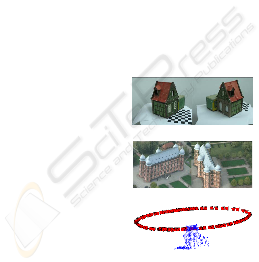
In Figure 1 and Figure 2, we present optical

images of a model house and of the Gottesaue Pa-

lace in Karlsruhe, Germany. The data set House was

reconstructed with 83 camera positions and some

10000 3D points. Bundle adjustment was run after

Euclidean reconstruction. The data set Gottesaue

was reconstructed with 339 camera positions and

some 40000 points.

Figure 3 and Figure 4 show the point clouds that

result from Step 1 of the procedure described in Sec.

2 above together with some of the camera positions.

Note the abruptly changing nature of the point cloud,

with adjacent sparse and dense regions. It is

particularly challenging to reconstruct the sparse

regions. In Figure 5 and Figure 6, we present the

scenes reconstructed and textured by the L

-spline-

based procedure of Sec. 2. Texturing was performed

using 594 and 1342 multipoints and 10 and 29

reference cameras for House and Gottesaue, res-

pectively. Note the sharp illumination changes in the

transition from the walls to the ground in the

colormap for Figure 6. In Figure 7 and Figure 8, we

show the triangular meshes and textured views of

buildings reconstructed by the conventional-spline-

based procedure described at the beginning of the

present section. Finally, in Figure 9 and Figure 10,

we present, for two characteristic values of α, the

meshes and final results for the buildings reconstruc-

ted and textured by the α-shapes procedure. The

computational results make clear the advantages of

the L

-spline-based procedure vs. the alternative pro-

cedures based on conventional splines and α-shapes.

Note by comparing Figure 6 and Figure 8 the nume-

rous extraneous, nonphysical peaks (oscillation) that

plague the conventional spline and the completeness

with which the L

spline eliminates these non-

physical peaks while retaining representation of

elevated physical objects such as the house beside

the palace on the left of Figure 2. Note also by

comparing Figure 6 with Figure 10 the inability of

α-shapes to produce a meaningful surface without

nonphysical holes when the data are noisy and

irregularly spaced and the ability of the L

spline to

produce an excellent, hole-free surface under the

same circumstances.

In the computational experiments for the sequen-

ce Gottesaue, the L

-spline-based procedure took

around 2 hours of computing time while the conven-

tional-spline-based and α-shapes-based procedures

took respectively about 1.5 and 0.5 minutes of com-

puting time. However, the quality of the reconstruct-

ed and textured scenes is inversely correlated to the

computing time. Even though the α-shapes-based

procedure performs rather well for the almost noise-

free data set House (Figure 9), it fails completely

when processing the noisy data set Gottesaue

(Figure 10) where no bundle adjustment took place.

The nonphysical oscillations near the gradient dis-

continuities and data outliers are quite apparent in

the results produced using conventional splines and

render these results difficult to accept.

Figure 1: Optical images from the sequence House.

Figure 2: Optical images from the sequence Gottesaue.

Figure 3: Point cloud for the sequence House together

with the camera trajectory.

VISAPP 2009 - International Conference on Computer Vision Theory and Applications

406

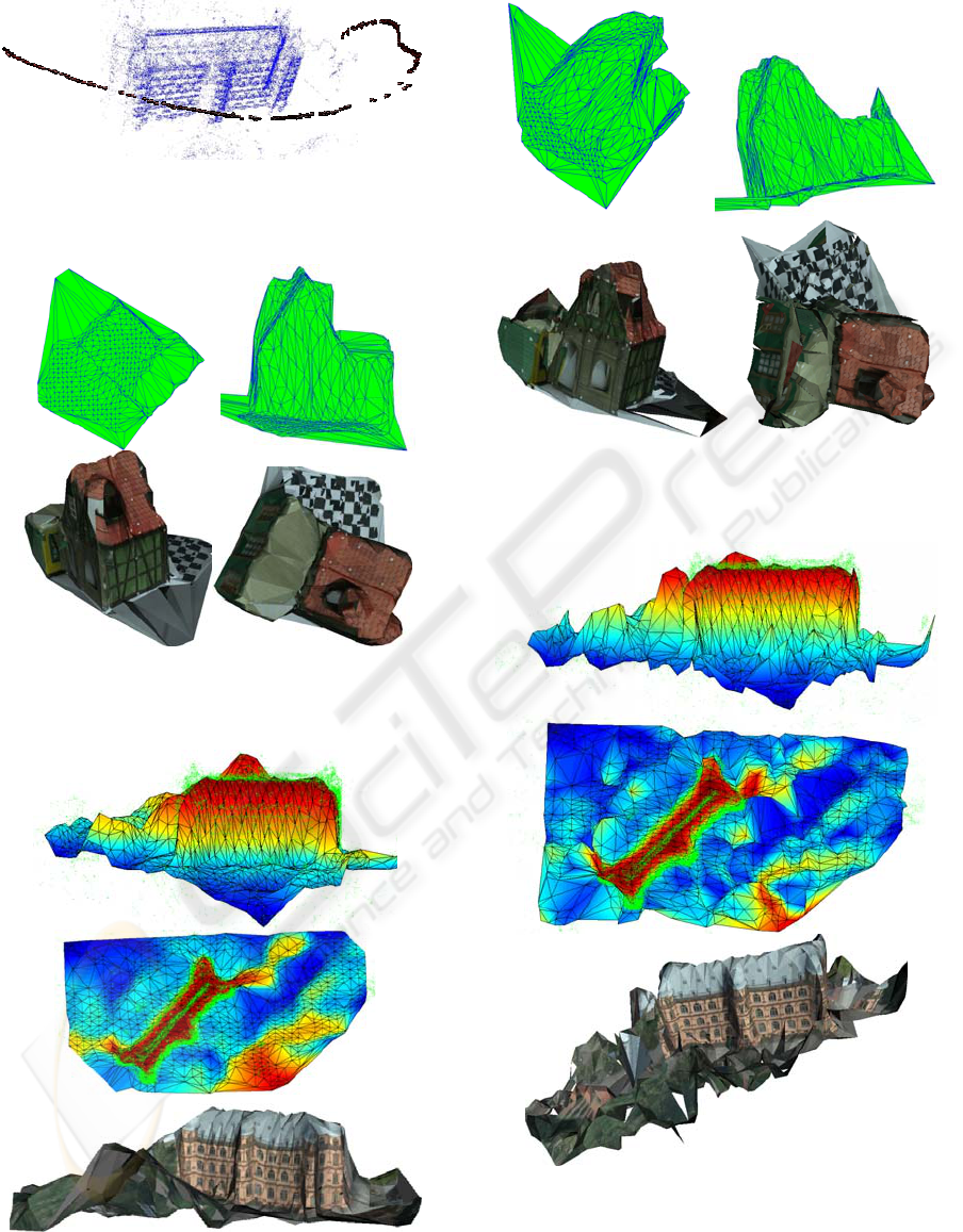
Figure 4: Point cloud for the sequence Gottesaue together

with a part of camera trajectory (placed artificially closer

to the point cloud).

Figure 5: Two views of the triangular mesh and two views

of the textured reconstruction produced from the sequence

House by the L

-spline-based procedure.

Figure 6: Two colormap views of the mesh and view of

the textured reconstruction produced from the sequence

Gottesaue by the L

-spline-based procedure. The original

point cloud is indicated by green points.

Figure 7: Two views of the triangular mesh and two views

of the textured reconstruction from the sequence House

produced by the conventional-spline-based procedure.

Figure 8: Two colormap views of the mesh and view of

the textured reconstruction produced from the sequence

Gottesaue by the conventional-spline-based procedure.

The original point cloud is indicated by green points.

COMPARISON OF RECONSTRUCTION AND TEXTURING OF 3D URBAN TERRAIN BY L1 SPLINES,

CONVENTIONAL SPLINES AND ALPHA SHAPES

407

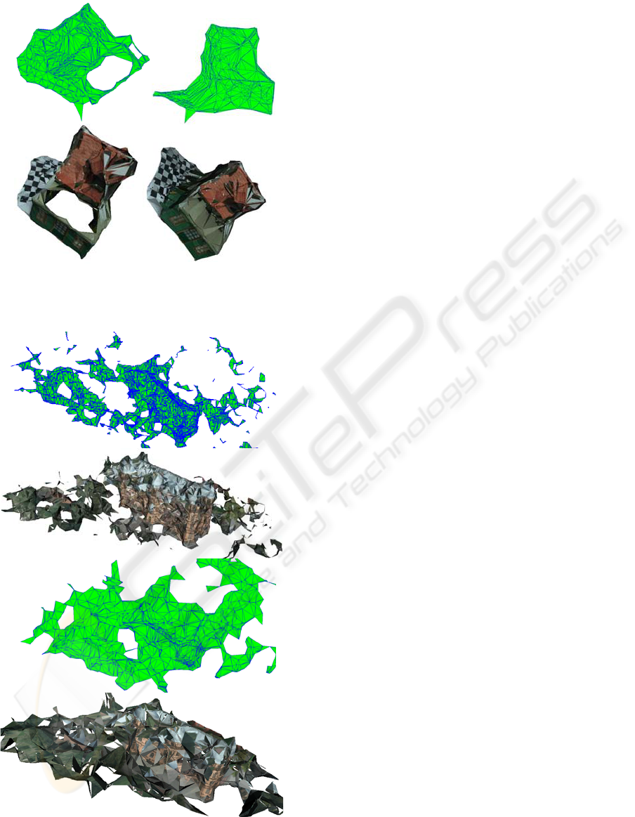
Figure 9: Two views of the mesh and of the textured re-

construction produced from the sequence House by the α-

shapes procedure. Left α = 1.0·10

σ, right α = 2.0·10

σ.

Figure 10: Views of the mesh and of the textured

reconstruction produced from the sequence Gottesaue by

the α-shapes-based procedure. α = 0.5·10

σ above and α =

2.0·10

σ below.

The high computing time of the L

-spline-based

procedure is an artifact of its current implementati-

on, which was designed to prove a principle rather

than to optimize computing time. The computing ti-

me can be reduced by 4 to 6 orders of magnitude by

using L

splines calculated by domain decomposi-

tion (Lin et al., 2006) rather than global splines,

improved gridding and improved software structure,

which will make the L

-spline-based procedure real-

time or nearly so. The enhanced accuracy that the

-spline-based procedure produces justifies expen-

ding the effort to make these improvements in the L

spline algorithm and software.

4 CONCLUSIONS AND FUTURE

WORK

The comparisons presented in this paper indicate

that the L

-spline-based procedure is an excellent

path to improving reconstruction and texturing of

urban terrain and is a significant advance over the

previous state of the art. This procedure is able to

handle abrupt changes in the density of the point clo-

ud and is able to produce excellent reconstructions

even in regions with sparse data. The comparisons

show the importance of using L

splines rather than

conventional splines and α-shapes for processing of

3D urban scenes.

Future work on terrain modeling will include im-

proved implementation of the L

-spline-based proce-

dure. In addition to improving the software structure

in general, we will parallelize the algorithm by

calculating multiple local L

splines instead of one

global spline (“domain decomposition”) and patch

together the global L

spline from these local splines.

This work will be an extension of work in (Lin et al.,

2006). We will also implement adaptive rectangular

and triangular grids that will assign data points to L

spline computational cells in an even manner, that is,

so that there are roughly equal numbers of data

points per cell throughout the domain. (At present, a

few cells contain the bulk of the data points and

many cells contain few or no data points, a situation

that arises from the unavoidably irregular nature of

the point cloud.) These changes will not merely

reduce the computing time by orders of magnitude

but will also allow further enhancement of the

accuracy of the textured reconstruction. With respect

to performance evaluation, we will carry out further

experiments for quantitative and qualitative eva-

luation of continuative modifications of the methods

described in this paper as well as other alternatives

for terrain modeling.

VISAPP 2009 - International Conference on Computer Vision Theory and Applications

408

REFERENCES

Bos, L. P., and Holland, D., 1996. Network splines,

Results Math. 30, 228–258.

Brovelli, M. A., and Cannata, M., 2004. Digital terrain

model reconstruction in urban areas from airborne

laser scanning data: the method and an example for

Pavia (northern Italy), Computers & Geosciences

30, 325–331.

Bulatov, D., 2008. Towards Euclidean reconstruction from

video sequences, Proc. VISAPP 2, 476–483.

Bulatov, D., and Lavery, J.E., 2009. Reconstruction and

texturing of 3D urban terrain from noisy optical data

using L

splines, to appear in Photogrammetric

Engineering and Remote Sensing.

Chui, C. K., 1988. Multivariate splines, Society for Indus-

trial and Applied Mathematics, Philadelphia.

Chui, C.K., Montefusco, L., and Puccio, L., (eds.), 1994,

Wavelets: Theory, algorithms and applications,

Academic Press.

Cressie, N. A., 1993. Statistics for spatial data, Wiley,

New York.

de Boor, C., 1993. Multivariate piecewise polynomials,

Acta Numerica 2, 65–109.

Edelsbrunner, D. and Mucke, E.P., 1994. Three-dimen-

sional α-shapes, ACM Trans. Graphics 13, 43–72.

Eck, M., and Hoppe, H., 1996. Automatic reconstruction

of B-spline surfaces of arbitrary topological type,

Proc. 23rd Annual Conf. Computer Graphics and

Interactive Techniques, 325–334.

Farin, G., 1995. NURB curves and surfaces, A.K. Peters,

Wellesley, MA.

Farin, G., 1997, Curves and surfaces for computer-aided

geometric design: A practical guide, 4th ed.,

Academic Press, San Diego.

Gilsinn, D. E., and Lavery, J. E., 2002. Shape-preserving,

multiscale fitting of bivariate data by cubic L

smoothing splines. In Approximation theory X:

Wavelets, splines, and applications (C.K. Chui, L.L.

Schumaker and J. Stöckler, editors), Vanderbilt

University Press, Nashville, Tennessee, 283–293.

Hartley, R. and Zisserman, A., 2000. Multi-view geometry

in computer vision, Cambridge University Press.

Lavery, J. E., 2001. Shape-preserving, multiscale inter-

polation by bi- and multivariate cubic L

splines,

Comput. Aided Geom. Design, 18, 321–343.

Lavery, J. E., 2004. The state of the art in shapepreserving,

multiscale modeling by L

splines, in M.L. Lucian and

M. Neamtu (Eds.), Proc. SIAM Conf. Geom. Design

Computing, Nashboro Press, Brentwood, TN, 2004,

365─376.

Lavery, J. E., 2006. Human-goal-based metrics for models

of urban and natural terrain and for approximation

theory,” Proc. 25th Army Science Conf. (November

2006), Department of the Army, Washington, DC

(2006), PO-01.

Lee, S., Wolberg, G., and Shin, S.Y., 1997. Scattered data

interpolation with multilevel B-splines, IEEE Trans.

Visual. Computer Graphics 3, 228–244.

Lin, Y.-M., Zhang, W., Wang, Y. Fang, S.-C., and Lavery,

J.E., 2006. Computationally efficient models of urban

and natural terrain by non-iterative domain

decomposition with L

smoothing splines, Proc. 25th

Army Science Conf. (November 2006), Department of

the Army, Washington, DC, PP-08.

Lucas B. and Kanade T., 1981. An iterative image re-

gistration technique with an application to stereo

vision. In Proceedings of 7th International Joint

Conference on Artificial Intelligence (IJCAI), 674-

679.

Martinec, D., Pajdla, T., Kostková, J., and Šara, R., 2006.

3D reconstruction by gluing pair-wise Euclidean

reconstructions, or “How to achieve a good

reconstruction from bad images”. Proc. 3D Data

Processing, Visualization and Transmission Conf.

(3DPVT), University of North Carolina, Chapel Hill,

USA.

Nistér, D., 2001. Automatic dense reconstruction from

uncalibrated video sequences, PhD Thesis, Royal

Institute of Technology KTH, Stockholm, Sweden.

Piegl, L. A., and Tiller, W., 1995. The book of NURBS,

Springer-Verlag, New York.

Powell, M. J. D., 1997. A new iterative algorithm for thin

plate spline interpolation in two dimensions, Ann.

Numer. Math. 4, 519–527.

Quak, E. and Schumaker, L. L., 1991. Least Squares

Fitting by Linear Splines on Data-Dependent

Triangulations, in Curves and Surfaces. P.J. Laurent.

A. LeMehaute. and L.L. Schumaker. eds., Academic

Press. New York, 387-390.

Späth, H., 1995. Two dimensional spline interpolation

algorithms, A.K. Peters, Wellesley, MA.

Thurston, J., 2003. Looking back and ahead: The triangu-

lated irregular network (TIN), GEOInformatics 6, 32–

35.

COMPARISON OF RECONSTRUCTION AND TEXTURING OF 3D URBAN TERRAIN BY L1 SPLINES,

CONVENTIONAL SPLINES AND ALPHA SHAPES

409