TOWARD LARGE SCALE MODEL CONSTRUCTION FOR
VISION-BASED GLOBAL LOCALISATION
P. Lothe, S. Bourgeois, F. Dekeyser
CEA, LIST, Boite Courrier 94, Gif-sur-Yvette, F-91191, France
E. Royer, M. Dhome
LASMEA UMR 6602, Universit
´
e Blaise Pascal/CNRS, Clermont-Ferrand, France
Keywords:
SLAM, 3D reconstruction, Non-rigid ICP, Global localisation, Trajectometry.
Abstract:
Monocular SLAM reconstruction algorithm advancements enable their integration in various applications: tra-
jectometry, 3D model reconstruction, etc. However proposed methods still have drift limitations when applied
to large-scale sequences. In this paper, we propose a post-processing algorithm which exploits a CAD model
to correct SLAM reconstructions. The presented method is based on a specific deformable transformations
model and then on an adapted non-rigid ICP between the reconstructed 3D point cloud and the known CAD
model. Experimental results on both synthetic and real sequences point out that the 3D scene geometry regains
its consistency and that the camera trajectory is improved: mean distance between the reconstructed cameras
and the ground truth is less than 1 meter on several hundreds of meters.
1 INTRODUCTION
Simultaneous Localization and Mapping (SLAM) and
Structure From Motion (SFM) methods enable to
reconstruct both the trajectory of a moving cam-
era and the environment. However, the first pro-
posed algorithms present a significant computation
burden which avoids large-scale sequence reconstruc-
tion. Recent works tend to overcome this limit by re-
ducing the problem complexity while still only using
easily embeddable and low-cost materials.
For example, Nister (Nister et al., 2004) does not
use any global optimisation. It enables him to speed
up the computation time but it is very sensitive to error
accumulations since the 3D scene geometry is never
questioned. Davison (Davison et al., 2007) proposes
a Kalman-filter based solution. This method reaches
real-time if the number of landmarks is quite small.
Another approach is to use a full non-linear optimi-
sation of the scene geometry: Royer (Royer et al.,
2005) uses a hierarchical bundle adjustment in order
to build large-scale scenes. Afterwards, Mouragnon
(Mouragnon et al., 2006) proposes an incremental
non-linear minimisation method in order to almost
completely avoid computer memory problem by only
optimizing the position of the geometry scene on the
few last cameras.
Nevertheless, monocular SLAM and SFM meth-
ods still present limitations: the trajectory and 3D
point cloud are known up to a similarity. Thus, all
the displacements and 3D positions are relative and
it is not possible to obtain an absolute localisation
of each reconstructed element. Besides, as well as
being prone to numerical errors accumulation (Davi-
son et al., 2007; Mouragnon et al., 2006), monocular
SLAM algorithms may present scale factor drift: their
reconstructions are done up to a scale factor, theoret-
ically constant on the whole sequence, but it appears
that it changes in practice. Even if these errors could
be tolerated for guidance applications which only use
local relative displacements, it becomes a burning is-
sue for other applications using SLAM reconstruction
results like trajectometry or global localization.
To improve SLAM results, a possible approach
consists in injecting a priori knowledge about the tra-
jectory (Levin and Szeliski, 2004) or about the envi-
ronment geometry (Sourimant et al., 2007). This last
kind of information can be provided by CAD models.
Furthermore, even if high precision models are still
unusual, coarse 3D city models are now wide spread
in GIS databases.
More precisely, we introduce in this paper a so-
429
Lothe P., Bourgeois S., Dekeyser F., Royer E. and Dhome M. (2009).
TOWARD LARGE SCALE MODEL CONSTRUCTION FOR VISION-BASED GLOBAL LOCALISATION.
In Proceedings of the Four th International Conference on Computer Vision Theory and Applications, pages 429-434
DOI: 10.5220/0001654204290434
Copyright
c
 SciTePress

lution which consists in estimating a non-rigid defor-
mation of the SLAM reconstruction with respect to
a coarse CAD model of the environment (i.e. only
composed of vertical planes representing buildings
fronts). First, a model of SLAM reconstruction er-
ror is used to establish a specific non-rigid transfor-
mations model of the reconstructed environment with
few degrees of freedom (section 2). Then, we esti-
mate the parameters of these transformations which
allow to fit the SLAM reconstruction on the CAD
model through a non-rigid ICP optimisation (sec-
tion 3). The complete refinement process is then eval-
uated on both synthetic and real sequences (section 4).
2 TRANSFORMATIONS MODEL
The registration of 3D point cloud and CAD model
has been widely studied. Main used methods are It-
erative Closest Point ICP (Rusinkiewicz and Levoy,
2001; Zhao et al., 2005) or Levenberg-Marquardt
(Fitzgibbon, 2001). Nevertheless, these methods only
work originally with Euclidean transformations or
similarities, what is not adapted to our problem. To
overcome with this limit, non-rigid fitting methods
have been proposed. Because of their high degree of
freedom, this category of algorithm needs to be con-
strained. For example (Castellani et al., 2007) use reg-
ularization terms to make his transformation be in ac-
cordance with his problem scope. Therefore we will
now introduce the specific non-rigid transformations
we use for our problem.
2.1 Non-Rigid Transformations Model
The constraints we used to limit the applicable trans-
formations on the 3D SLAM reconstruction are based
on experimental results. We observe that the scale
factor is nearly constant on straight lines trajectory
and change during turnings (see figure 5(b)). So we
have decided to consider trajectory straight lines as
rigid body while articulations are put in place in each
turning. Thus the selected transformations are piece-
wise similarities with joint extremities constraints.
Thus, the first step is to automatically segment our
reconstructed trajectory. We use the idea suggested
by Lowe in (Lowe, 1987). He proposes to cut re-
cursively a set of points into segments with respect
both to their length and their deviation. So we split
the reconstructed trajectory (represented as a set of
temporally ordered key cameras) into m different seg-
ments (T
i
)
1≤i≤m
whose extremities are cameras de-
noted (e
i
, e
i+1
).
2.2 Transformations Parametrisation
Once the trajectory is split into segments, each 3D re-
constructed point must be associated to one cameras
segment. We say that a segment “sees” a 3D point
if at least one camera of the segment observes this
point. There are two cases for point-segment associ-
ation. The simplest is when only one segment sees
this point: the point is then linked to this segment.
The second appears when a point is seen by two or
more different segments. In this case, we have tested
different policies which give the same results and we
arbitrarily decided to associate the point to the last
segment which sees it.
We call B
i
a fragment composed both of the cam-
eras of T
i
(i.e. those included between e
i
and e
i+1
)
and of the associated reconstructed 3D points. Obvi-
ously, for 2 ≤ i ≤ m − 1, the fragment B
i
shares its
extremities with its neighbours B
i−1
and B
i+1
.
We saw in section 2.1 that applied transforma-
tions are piecewise similarities with joint extremities.
Practically, those transformations are parametrized
with the 3D translation of the extremities (e
i
)
1≤i≤m+1
.
From these translations, we will deduce the similari-
ties to apply to each fragment (i.e. its cameras and
3D points). Precisely, since camera is embedded on
a land vehicle, the roll angle is not called into ques-
tion. Then, each extremity e
i
has 3 degrees of free-
dom and so each fragment has 6 degrees of freedom
as expected.
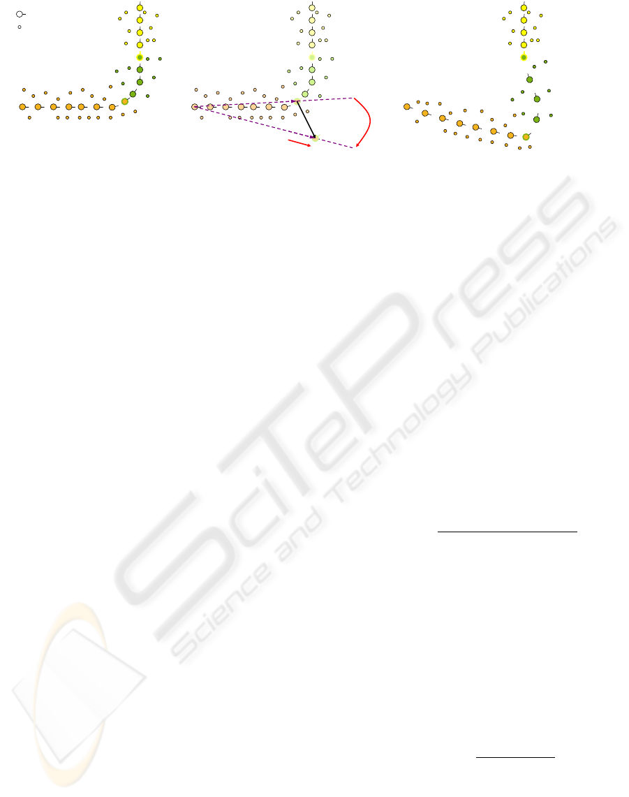
Figure 1 presents an example of extremity dis-
placement.
3 NON-RIGID ICP
Once we have defined the used non-rigid transfor-
mations (section 2.1) and their parametrisation (sec-
tion 2.2), we can use additional information provided
by CAD model to improve the SLAM reconstruction.
Thus, we propose in this part a non-rigid ICP between
the reconstructed 3D point cloud and CAD model:
first we present the cost function we minimize, the
different optimization steps and then parameters ini-
tialisation.
Cost Function. Once all the pre-treatment steps are
done, we dispose of both the fragmented reconstruc-
tion and a simple coarse 3D model of the scene.
In our work, we want to fit the 3D point cloud onto
the CAD model. The base cost function ε is then the
normal distance d between a 3D point and the CAD
model M , i.e. the distance between a 3D point Q
i
and
VISAPP 2009 - International Conference on Computer Vision Theory and Applications
430

Key camera
Reconstructed 3D
point
e
i−1
e
i
e
i+1
e
i+2
(a)
t
R
s
e
i−1
e
i
e
i+1
e
i+2
e
0
i
(b)
e
i−1
e
0
i
e
i+1
e
i+2
(c)
Figure 1: An example of fragment-based reconstruction transformation. (a) The segmentation of the original reconstruc-
tion. (b) A 3D translation of the extremity e
i
. The similarity S(e
i−1
, s, R ) is then deduced from this 3D displacement and
applied to the whole fragment B
i−1
. An equivalent treatment is realized on B
i
. (c) The result of the transformation: the two
fragments linked to the moved extremity have been modified.
the plane P
g
i
it belongs to:
ε(Q
i
, M ) = d(Q
i
, M )
= d(Q
i
, P
g
i
) (1)
Non-linear Minimization. The aim of this step is
to transform the different fragments to minimise the
distance between the reconstructed point cloud and
the CAD model, i.e. solving the problem:
min
e
1
,...,e
m+1
∑
i
d(Q
i
, M )
2
(2)
Point-Plane Association. The problem in point-
plane association is that we do not know in reality on
which CAD model plane P
g
i
belongs each 3D recon-
structed point. So we make the hypothesis that it is
the nearest one. Equation 1 becomes:
ε(Q
i
, M ) = min
P
j
∈M
d(Q
i
, P
j
) (3)
Furthermore, to reduce algorithm complexity, we
consider that for a point Q
i
, the nearest plane P
h
i
does
not change during the minimization. Thus, the selec-
tion between 3D point and corresponding plane can
be done outside the minimization:
∀Q
i
, P
h
i
= argmin
P ∈M
d(Q
i
, P ) (4)
Besides, the distance d takes into account that the
planes are finite: to be associated to a plane P , a
3D point Q must have its normal projection inside P
bounds.
Robust Estimation. There are two cases where the
association (Q
i
, P
h
i
) can be wrong: if the initial posi-
tion of Q
i
is too far from its real position or if it is not
(in the real scene) on the CAD model. In those two
cases, d(Q
i
, P
h
i
) could make the minimization fail. To
limit this effect, we insert a robust M-estimator ρ in
equation (2):
min
e
1
,...,e
m
∑
i
ρ(d(Q
i
, P
h
i
)) (5)
We chose to use the Tukey M-estimator (Huber,
1981). The M-estimator threshold can be automati-
cally fixed thanks to the Median Absolute Deviation
(MAD). The MAD works with the hypothesis that the
studied data follow a Gaussian distribution around the
model. This assumption could be done for each indi-
vidual fragment but not for the whole reconstruction.
So we decided to use a different M-estimator thresh-
old ξ
j
per fragment. This implies that we have to nor-
malize the Tukey values on each fragment:
ρ
0
l
i
(d(Q
i
, P
h
i
)) =
ρ
l
i
(d(Q
i
, P
h
i
))
max
Q
j
∈B
l
i
ρ
l
i
(d(Q
j
, P
h
j
))
(6)
where l
i
is the index of the fragment owning Q
i
and ρ
l
i
the Tukey M-estimateur used with the threshold ξ
l
i
.
Fragment Weighting. With this cost function, each
fragment will have a weight in the minimization pro-
portional to the number of 3D points it contains.
Then, fragments with few points could be not opti-
mize in favour of the others. To give the same weight
to each fragment, we must unified all the Tukey val-
ues of their 3D points with respect to their cardinal:
ρ
∗
l
i
(d(Q
i
, P
h
i
)) =
ρ
0
l
i
(d(Q
i
, P
h
i
))
card(B
l
i
)
(7)
and the final minimization problem is:
min
e
1
,...,e
m+1
∑
i
ρ
∗
l
i
(d(Q
i
, P
h
i
)) (8)
that we solve using the Levenberg-Marquardt algo-
rithm (Levenberg, 1944).
TOWARD LARGE SCALE MODEL CONSTRUCTION FOR VISION-BASED GLOBAL LOCALISATION
431

Iterative Optimisation. Practically, several non-
linear minimisations are done successively with com-
puting the point-plane association before each one of
them. It enables 3D points to change their associated
plane without losing cost-function computation time.
Initialisation. Non-linear algorithms require a cor-
rect initialisation: the 3D reconstruction should be
placed in the same frame than the CAD model. To re-
alize this stage, estimating an initial rigid transforma-
tion is sufficient when the 3D reconstruction is accu-
rate. However, the drift of the scale factor frequently
observed with SLAM reconstruction may induce im-
portant geometrical deformations. Therefore, to en-
sure convergence of the algorithm, we chose to place
roughly each extremity e
i
around the CAD model. It
can be done automatically if the sequence is synchro-
nised with GPS data for example. Otherwise, it could
be realized manually through graphic interface.
4 EXPERIMENTAL RESULTS
In this part, we will present results on both synthetic
and real sequences. The SLAM algorithm we use for
our reconstruction is the one proposed by Mouragnon
(Mouragnon et al., 2006).
4.1 Synthetic Sequence
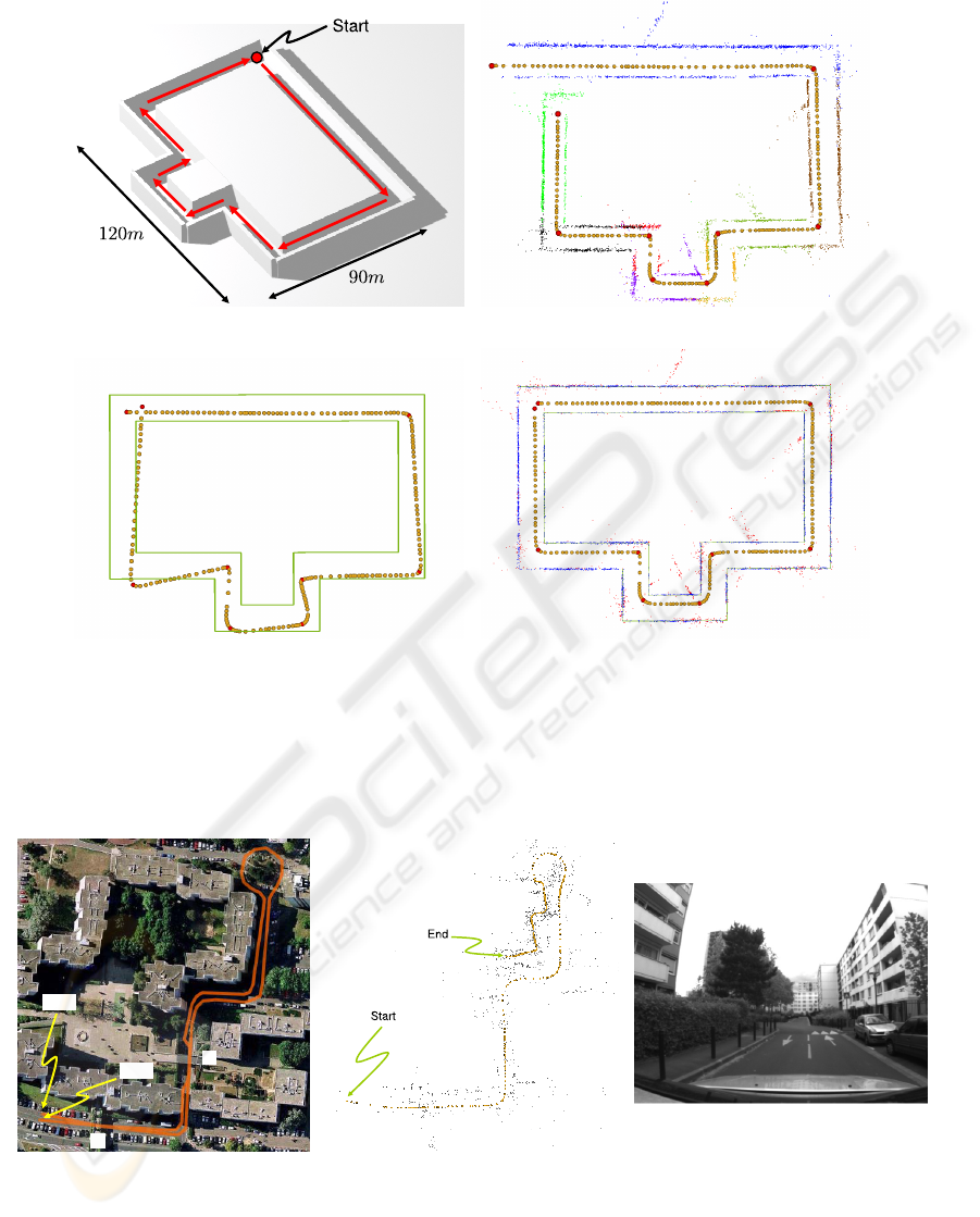
Figure 4 presents the different steps of our experi-
ment. The synthetic sequence (based on 3D model
figure 4(a)) have been made by using the SLAM al-
gorithm in a textured 3D world generated with a 3D
computer graphics software. The followed trajectory
is represented by the red arrows in figure 4(a).
Table 1: Numerical results on the synthetic sequence.
Each value is a mean over all the reconstruction.
Before ICP After ICP
Camera distance
to ground truth (m)
4.61 0.51
Standard Deviation (m) 2.25 0.59
3D points-Model
distance (m)
3.37 0.11
Standard Deviation (m) 3.9 0.08
Tukey threshold × 0.38
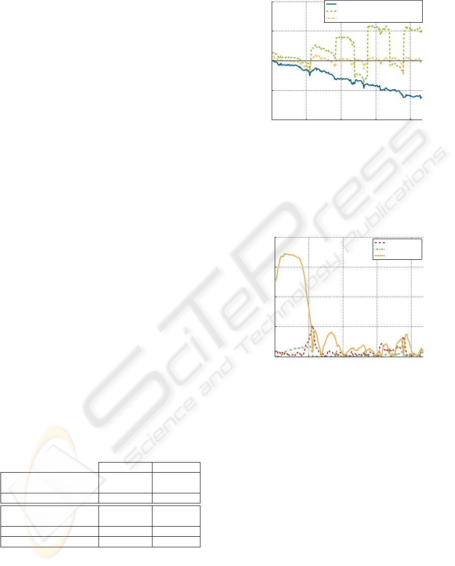
Figure 2 underlines the original SLAM method
drift. The scale factor is measured by computing the
distance between two successive cameras and then
computing the ratio for ground truth and reconstruc-
tion results. We see that this scale factor decreases
in the course of the journey, making the 3D SLAM
0 50 100 150 200
0.5
0.75
1
1.25
1.5
Trajectory (key cameras)
Scale factor compared to ground truth
SLAM reconstruction (normalised)
Manual initialisation
Our method result
Figure 2: Scale factor evolution. We can observe the scale
factor drift on the original SLAM reconstruction. After our
method, scale factor is centred around 1.
reconstruction being distorted (figure 4(b)). As con-
sequence, the camera trajectory does not loop any-
more. For ICP initialisation, we have manually sim-
0 50 100 150 200
0
0.5
1
1.5
2
Trajectory (key cameras)
Distance between reconstructed
and ground truth cameras (m)
Distances in X
Distances in Y
Distances in Z
Figure 3: Residual values on distances between recon-
structed cameras and ground truth. The (X, Y, Z) coor-
dinates frame is relative to each camera : Z is the optical
axis, X is the latitude axis and Y the altitude.
ulated GPS results: random position error have been
assigned to each extremity (figure 4(c)).
Then we observe that after our treatment (fig-
ure 4(d)) the loop is restored while no loop constraint
is directly included into our transformation model.
Besides the 3D reconstructed point cloud regains its
consistency. Table 1 confirms those enhancements:
the average distance between the reconstructed cam-
eras and the ground truth is reduced from more than
4 meters to about 50 centimetres. Statistics before
ICP have been computed on the 5591 reconstructed
3D points (among the 6848 proposed by SLAM) kept
as inliers by the ICP step. Furthermore, we can notice
in figure 3 that only errors along the direction of the
trajectory remain significant. This is due to the fact
that we have supposed the error on scale factor strictly
VISAPP 2009 - International Conference on Computer Vision Theory and Applications
432

(a) (b)
(c) (d)
Figure 4: Synthetic sequence treatment. (a) Synthetic 3D model. (b) Top view of its 3D reconstruction with (Mouragnon
et al., 2006) algorithm. Orange spheres are cameras while red ones are the fragment extremities. The automatic trajectory
and point-fragment segmentation is also represented: the reconstructed 3D points are coloured by fragment belonging. Figure
(c) is the user initialisation of the trajectory around the CAD model (in green) before the ICP step. Figure (d) shows the 3D
reconstruction after our method: blue 3D points are inliers and red are outliers.
A
B
Start
End
(a) (b) (c)
Figure 5: Real sequence reconstruction using (Mouragnon et al., 2006). (a) is a satellite map of the reconstructed trajectory
displayed in (b). (c) is a frame of the video sequence.
TOWARD LARGE SCALE MODEL CONSTRUCTION FOR VISION-BASED GLOBAL LOCALISATION
433

constant on each segment. Although this hypothesis
reveals to be only a rough approximation.
4.2 Real Sequence
The real sequence (figure 5) is a about 600m long
loop. The SLAM reconstruction (figure 5(b)) is a
good example of scale factor drift: we can see that
after the roundabout, there is a radical change of scale
factor and then the loop is not respected.
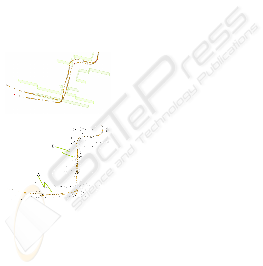
Since no ground truth is available for this se-
quence, we can only have a visual appreciation of our
results. Nevertheless, two recognizable places in fig-
ures 5(a) and 6(b) tend to point out our method con-
sistency: we find in “A” a crossroad due to a single
way tunnel. Besides, in “B” we can show that we pass
twice on the same lane because of a car breakdown.
(a)
(b)
Figure 6: Real sequence treatment. (a) ICP initialisation
for real sequence. (b) Correction of real sequence recon-
struction thanks to our method. “A” and “B” correspond to
“A” and “B” places in figure 5(a).
5 CONCLUSIONS
We have presented in this paper a post-processing al-
gorithm that improves SLAM reconstruction. Our
method uses an automatic fragmentation of the re-
constructed scene and then a non-rigid ICP between
SLAM reconstruction and a coarse CAD model of the
environment. Synthetic and real experiments point
out that method can clearly reduced the 3D positions
error, in particular in X and Y directions: trajectory
loop are restored and cameras position errors are re-
duced to about 50 centimetres on several hundreds
meters sequences.
To improve our method, it would be interesting to
evaluate the performance of an automatic initialisa-
tion (which could be provided by an additional sensor:
GPS for example). We are also working on further re-
finements of the reconstruction by including the CAD
model information into a bundle adjustment process.
REFERENCES
Castellani, U., Gay-Bellile, V., and Bartoli, A. (2007). Joint
reconstruction and registration of a deformable planar
surface observed by a 3d sensor. In 3DIM, pages 201–
208.
Davison, A., Reid, I., Molton, N., and Stasse, O. (2007).
MonoSLAM: Real-time single camera SLAM. PAMI,
26(6):1052–1067.
Fitzgibbon, A. (2001). Robust registration of 2d and 3d
point sets. In BMVC, pages 411–420.
Huber, P. (1981). Robust Statistics. Wiley, New-York.
Levenberg, K. (1944). A method for the solution of cer-
tain non-linear problems in least squares. Quart. Appl.
Math., 2:164–168.
Levin, A. and Szeliski, R. (2004). Visual odometry and map
correlation. In CVPR, pages 611–618.
Lowe, D. G. (1987). Three-dimensional object recognition
from single two-dimensional images. Artificial Intel-
ligence, 31(3):355–395.
Mouragnon, E., Dekeyser, F., Sayd, P., Lhuillier, M., and
Dhome, M. (2006). Real time localization and 3d re-
construction. In CVPR, pages 363–370.
Nister, D., Naroditsky, O., and Bergen, J. (2004). Visual
odometry. In CVPR, pages 652–659.
Royer, E., Lhuillier, M., Dhome, M., and Chateau, T.
(2005). Localization in urban environments: Monoc-
ular vision compared to a differential gps sensor. In
CVPR, pages 114–121.
Rusinkiewicz, S. and Levoy, M. (2001). Efficient variants
of the ICP algorithm. In 3DIM, pages 145–152.
Sourimant, G., Morin, L., and Bouatouch, K. (2007). Gps,
gis and video fusion for urban modeling. In CGI.
Zhao, W., Nister, D., and Hsu, S. (2005). Alignment
of continuous video onto 3d point clouds. PAMI,
27(8):1305–1318.
VISAPP 2009 - International Conference on Computer Vision Theory and Applications
434