USING THE STOCHASTIC APPROACH FRAMEWORK TO MODEL
LARGE SCALE MANUFACTURING PROCESSES
Benayadi Nabil, Le Goc Marc
LSIS, Laboratory for Information and System Sciences,University of Marseilles, Marseilles, France
Bouch´e Philippe
LGECO, INSA de Strasbourg, Strasbourg, France
Keywords:
Information-Theory, Temporal Knowledge Discovering, Chronicles Models, Markov Processes.
Abstract:
Modelling manufacturing process of complex products like electronic ships is crucial to maximize the quality
of the production. The Process Mining methods developed since a decade aims at modelling such manufac-
turing process from the timed messages contained in the database of the supervision system of this process.
Such process can complex making difficult to apply the usual Process Mining algorithms. This paper proposes
to apply the Stochastic Approach framework to model large scale manufacturing processes. A series of timed
messages is considered as a sequence of class occurrences and is represented with a Markov chain from which
models are deduced with an abductive reasoning. Because sequences can be very long, a notion of process
phase based on a concept of class of equivalence is defined to cut up the sequences so that a model of a phase
can be locally produced. The model of the whole manufacturing process is then obtained with the concate-
nation of the model of the different phases. The paper presents the application of this method to model the
electronics chips manufacturing process of the STMicroelectronics Company (France).
1 INTRODUCTION
1
Modeling manufacturing process of complex ob-
jects like electronic ships is crucial to minimize the
scrapped objects and so to maximize the production
of objects. The methods and the algorithms developed
in the ”Process Mining” domain aims at modeling
such manufacturing process with a graph of manufac-
turing steps (treatments, operations or tasks) from the
timed messages contained in the database. (Cook and
Wolf, 1998). The proposed algorithms generally gen-
erate complex model so that they are difficult to use
when the manufacturing process contains hundreds of
steps. This paper proposes a modeling method and
the corresponding algorithms to model manufactur-
ing processes having hundreds of steps. The proposed
method is based on the cutting up of the sequences in
sub-sequences called process phases where there is
no cycle. The corresponding hypothesis is that when
a subsequence contains two occurrences of the same
step S made on the same machine but at two different
1
This study has been made possible thanks to the finan-
cial support of STMicroelectronics Company (France).
times, the product is not in the same state: there is
then a priori no relations between the series of steps
following the first step S and the series of steps fol-
lowing the second steps S. So the two series must be
represented with two different models.
The section 2 recalls briefly the main approaches
of the Process Mining area and the main characteris-
tics of the Stochastic Approach framework. Section
3 defines the notions of class of equivalence and pro-
cess phase that we propose and describes the algo-
rithms that are required to this aim. Section 4 presents
the application of the algorithms to model the manu-
facturing process of wafers (i.e. silicon plates where
electronic ships are engraved) of the Rousset (France)
plant of the STMicroelectronics Company. The paper
concludes in section 5 with a summary of the pro-
posed method and introduces of our current works.
2 RELATED WORKS
In the Process Mining framework, a series of mes-
sages is considered as an ordered set of events from
186
Nabil B., Goc Marc L. and Philippe B. (2008).
USING THE STOCHASTIC APPROACH FRAMEWORK TO MODEL LARGE SCALE MANUFACTURING PROCESSES.
In Proceedings of the Third International Conference on Software and Data Technologies - ISDM/ABF, pages 186-191
DOI: 10.5220/0001888801860191
Copyright
c
 SciTePress

which a process model is to be inferred and repre-
sented with a formalism (workflows, state charts or
Petri nets for examples) (van der Aalst and Weijters,
2004). One of the first algorithm was proposed in
(Agrawal et al., 1998). The algorithm aims at find-
ing workflow graphs from a set of series of events
contained in a workflow log. An event represents the
start time of a task. To avoid the problem of poten-
tial cycles (i.e. repeated events in a series), the algo-
rithm first renames the repeated labels of task before
enumerating the binary dependencyrelations between
the tasks. This set of relations is then reduced with the
use of the transitivity property of the binary relations.
Labels are again renamed to merge the tasks, making
possible the introduction of cycles in the model. Dif-
ficulties arise with this approach when (i) the tasks are
statistically independent and (ii) the number of tasks
is large (Agrawal et al., 1998). Nevertheless, Pinter
(Pinter and Golani, 2004) extends this algorithm no-
tably with the introduction of events marking the end
of the tasks. Similar issues in the context of software
engineering processes are investigated in (Cook and
Wolf, 1998) where the aim is to build a finite state
machine from the set of the most frequent event pat-
terns mined in a given log. In particular, the Markov
algorithm is based on a two order Markov chain that
is converted in states and state transitions. Cook and
Wolf (Cook and Wolf, 2004) extend this method to
concurrent processes and uses a first order Markov
chain to this aim. The difficulties come from the
pruning of the finite state machine to obtain a mini-
mal model and the sensibility of pruning metrics to
the ”noise” (van der Aalst and Weijters, 2004). Aalst
(van der Aalst et al., 2004) defines the class of process
that can be modeled with the α-algorithm but this al-
gorithm requires the series of events in the log to be
noise-free and complete.
There is a consensus to consider that finite state ma-
chines are difficult to understand and to validate. And
most of the proposed methods have difficulties when
(i) the process contains a lot of steps, (ii) the series in
the log induce potential cycles in the models and (iii)
the sequences are not noise-free and complete. The
Stochastic Approach framework (Le Goc et al., 2005)
for discovering temporal knowledge from timed ob-
servations provides a general frameworkfor modeling
dynamic processes that is based on a markovianrepre-
sentation but uses abstract chronicle models (Ghallab,
1996) instead of finite state machines. This frame-
work considers that the timed messages of a series are
written in a database by a program, called a monitor-
ing cognitive agent MCA, that monitors a production
process Pr. A timed message is represented with an
occurrence of a discrete event class C
i
= {e
i
} that is
an arbitrary set of discrete event e
i
= (x
i
, δ
i
), where δ
i
is one of the discrete value of the variable x
i
. When
the variable x
i
is not known, an abstract variable φ
i
is used to define the discrete event e
i
= (φ
i
, δ
i
) cor-
responding to the constant δ
i
. A discrete event class
is often a singleton because in that case, two discrete
event classes C
i
= {(x
i
, δ
i
)} and C
j
= {(x
j
, δ
j
)} are
only linked with the variables x
i
and x
j
when the con-
stants δ
i
and δ
j
are independent (Le Goc, 2006). This
condition is only concerned with the programs the
MCA is made with. A sequence of discrete event
class occurrences is then considered as the observ-
able manifestation of a series of state transitions in
a timed stochastic automaton representing the cou-
ple (Pr, MCA). The BJT4G algorithm represents a
set of sequences of discrete event class occurrences
with a one order Markov chain and uses an abduc-
tive reasoning to identify the set of the most proba-
ble timed sequential binary relations between discrete
event classes leading to a given class. A timed se-
quential binary relation R(C
i
,C
j
, [τ
−
ij
, τ
+
ij
]) is an ori-
ented relation between two discrete event classes C
i
and C
j
that is timed constrained with the interval
[τ
−
ij
, τ
+
ij
]. [τ
−
i, j
, τ
+
i, j
] is the time interval for observing
an occurrence of the C
j
class after an occurrence of
the C
i
class. The set of timed sequential binary rela-
tion is an abstract chronicles model that is graphically
represented with the ELP language (Event Language
for Process) where the nodes are discrete event classes
and the links are timed sequential binary relations. In
this paper, we propose to tackle the two main prob-
lems of the Process Mining approaches with the ex-
tension of the Stochastic Approach framework.
3 EXTENSION OF THE
STOCHASTIC APPROACH FOR
PROCESS MINING
3.1 Motivation
Let us take an example to illustrate the proposed ex-
tensions with a manufacturing process having a set
S = {A, B,C, D, E} of 5 manufacturing steps. Sup-
pose the supervision system records the execution of
a step with a message X(t
k
) denoting the time t
k
of the
beginning of the execution of the step X. The three
series of messages of table 1 is represented with the
abstract chronicle model of figure 1. In this model, if
the two nodes labeled with A denote the same manu-
facturing step, then the two nodes must be confused,
introducing a cycle in the model. The same reasoning
must be done with the other nodes, making the model
USING THE STOCHASTIC APPROACH FRAMEWORK TO MODEL LARGE SCALE MANUFACTURING
PROCESSES
187

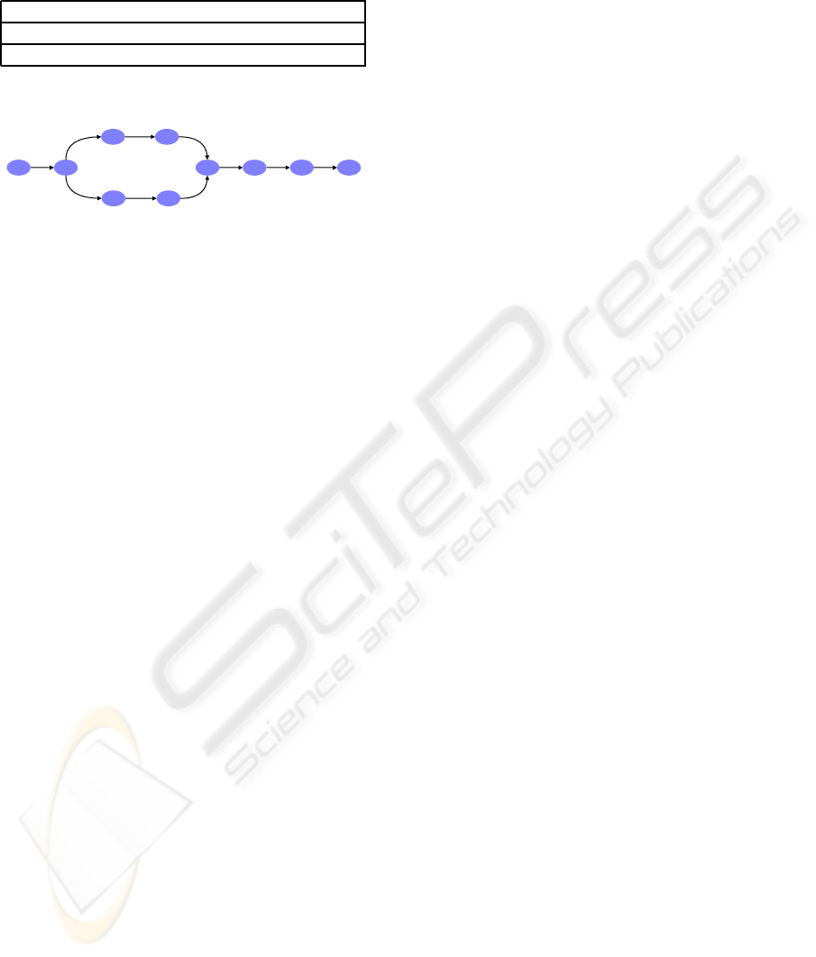
difficult to read and to understand.
Table 1: Three series of event.
A(t
1
)B(t
2
)D(t
3
)C(t
4
)E(t
5
)A(t
6
)E(t
7
)B(t
8
)
A(t
9
)B(t
10
)C(t
11
)D(t
12
)E(t
13
)A(t
14
)E(t
15
)B(t
16
)
A(t
17
)B(t
18
)C(t
19
)D(t
20
)E(t
21
)A(t
22
)E(t
23
)B(t
24
)
C
BA A E B
D
E
[
τ
A,B

,τ
A,B

]
[
τ
B,C

,τ
B,C

]
[
τ
D,C

,τ
D,C

]
[
τ
D,E

,τ
D,E

]
[
τ
C,E

,τ
C,E

]
[
τ
A,E

,τ
A,E

]
[
τ
E,B

,τ
E,B

][
τ
E,A

,τ
E,A

]
D
[
τ
B,D

,τ
B,D

]
C
[
τ
C,D

,τ
C,D

]
Figure 1: Model for the three Sequences.
Suppose now that each of the three sequences is
cut up when a label appears two times. The model of
the first part of the sequences will be similar to the one
of figure 1 but without the path A− E − B at the end
of the model: the steps A, B and E introduce no more
cycle. This fact motivates the notion of process phase
proposed in this paper. But this notion is not sufficient
to solve the cycles that are introduced with the steps C
and D. We consider that this problem is due to the fact
that the three series of events provide no information
about the order of the steps C and D. Consequently,
any solution of this problem must take into account
some a priori knowledge about the process which we
want to avoid it. The notion of potential cycle is then
defined to detect this kind of situation to be able to
make further investigations (i.e. finding new series or
discussing with experts for examples).
To illustrate the notion of class of equivalence, let
us take the Edit activity of the ”writing a scientific pa-
per” process that can be made by different students
and professors. The Edit activities can then be la-
beled differently according to the performer with a set
of classes of the form: C = {C
E1
= {(s
1
, δ
1
)},C
E2
=
{(s
2
, δ
2
)}, . . .}, where the variables s
i
and p
i
denotes
respectively students and professors. In this case, the
resulting model of the process will be complex with-
out necessity. One of the interesting features of the
Stochastic Approach framework is the notion of dis-
crete event class. This notion can be used to define ab-
stract classes of the form C
φ
i
= {(φ
i
, δ
1
), . . . , (φ
i
, δ
n
)}
where φ
i
denotes an abstract variable and the set
{δ
j
}, j = 1. . . n, is an arbitrary set of constants. This
property allows defining classes of equivalence that
simplifies a process model. For example, an abstract
class C
φ
i
be defined as an equivalent class of the set of
classes C of the ”writing a scientific paper” process.
Doing this way allows constituting a set of sequences
coming from different students and professors.
3.2 Class of Equivalence
By definition, a large scale process is made with a lot
of steps. Some of these steps differs only with some
characteristics but realizes similar treatments.
Definition 1
. Given a model M =
{R(C
i
,C
j
, [τ
−
i
j
, τ
+
ij
])} build with a set Ω = {ω
i
}
of discrete event class occurrences ω
i
, a class
C
φ
i
= {(φ
i
, δ
1
), (φ
i
, δ
2
), . . . , (φ
i
, δ
n
)} is an equiv-
alence class of a sub set of classes C = {C
j
},
j = 1. . . n, C
j
= {(x
j
, δ
j
)}, of the set of classes C
M
of
a model M iff:
∀C
j
∈ C, ∃R(C
i
,C
j
, [τ
−
ij
, τ
+
ij
]) ∈ M
∧∃R(C
j
,C
k
, [τ
−
jk
, τ
+
jk
]) ∈ M (1)
This definition means that every classes C
j
of the
sub set C ⊆ C
M
are linked with the same classes
in M. When this condition is verified, each oc-
currences C
j
(k) of the classes C
j
in the sequences
ω
i
of Ω can be rewritten as occurrences C
φ
i
(k)
of the equivalence class C
φ
i
. The abstract vari-
able φ
i
has no a priori meaning: φ
i
can be substi-
tuted with the corresponding concrete variable x
i
in
any occurrences C
φ
i
(k). Consequently, the set of
uphill relations {R(C
i
,C
j
, [τ
−
ij
, τ
+
ij
])} of M will be-
come {R(C
i
,C
φ
i
, [τ
−
iφ
i
, τ
+
iφ
i
])} and the set of down-
hill relations {R(C
j
,C
k
, [τ
−
jk
, τ
+
jk
])} of M will become
{R(C
φ
i
,C
k
, [τ
−
φ
i
k
, τ
+
φ
i
k
])}. In practice, an equivalence
class can be used to represent discrete event classes
having similar meanings. In the application presented
in the next section, a discrete event class represents
a treatment made on a product with a particular ma-
chine. Equivalence classes are then used to represent
the same treatment made on different machines: in
that case, the machines are equivalents because the
same treatment can be done on each of the machines.
Given a set of sequences Ω = {ω
i
}, the algorithm
for defining equivalence classes find all the equiv-
alence classes and rewrite the corresponding occur-
rences in each sequence ω
i
(Algorithm 1):
1. Build a model M given a set Ω of sequences ω
i
2. Find all the subset of classes C = {C
j
} verifying
the equation 1
3. For all the sub sets C
• Create an equivalence class C
φ
i
.
• For all C
j
∈ C, rewrite all the occurrencesC
j
(k)
in all the sequences ω
i
⊂ Ω with the rewriting
rule: C
j
(k) ≡ C
φ
i
(k).
4. Build a new model M
′
with Ω.
ICSOFT 2008 - International Conference on Software and Data Technologies
188

3.3 Process Phase
The information contained in a series of manufactur-
ing messages is concerned both with the state of the
manufactured object and the manufacturing process
that make evolving this state from an initial state up
to a final state. But generally, the state of the manu-
factured object is not provided with the messages. So
we propose to capture indirectly this dimension with
the notion of process phase.
Definition 2
. A process phase is a sub model M
′
=
{R(C
i
,C
j
, [τ
−
i
j
, τ
+
ij
])} so that there is no path P =
{R(C
i
,C
i+1
, [τ
−
ii+1
, τ
+
ii+1
])} ∈ M
′
, i = 1. . . n, where:
∀i < j ≤ n+ 1,C
i
= C
j
(2)
A process phase is then a sub model that does not
contain two times the same discrete event class. The
algorithm 2 aims at cutting up a set Ω of sequences
ω
i
in sub sequences ω
i
k
that respects the equation 2
(i.e. ω
i
k
does not contain two occurrences of the same
class):
1. ∀ω
i
∈ Ω do
• Remove ω
i
from Ω.
• Cut up ω
i
in a set Ω
i
= {ω
i
k
} of sub sequences
ω
i
k
verifying the equation 2.
2. ∀ω
i
k
∈ Ω
i
do
• Add an occurrence of the C
0
and C
1
classes at
the beginning and the end of ω
i
k
3. Ω =
S
Ω
i
.
An occurrence of an abstract start class C
0
and
an occurrence of an abstract final class C
1
are added
at the beginning and the end of each sub sequences
ω
i
k
so that the BJT4G algorithm automatically iden-
tifies the process phases. For example, when ap-
plying the algorithm 2 on the three sequences of
Table 1, the BJT4G algorithm will find two pro-
cess phases: the first phase starts from the event
class C
A
and finishes at the first event class C
E
,
the algorithm add the start class C
0
and finish class
C
1
at this phase. The second process phase be-
ing: { R(C
0
,C
A
, [τ
−
0A
, τ
+
0A
]) , R(C
A
,C
E
, [τ
−
AE
, τ
+
AE
]),
R(C
E
,C
B
, [τ
−
EB
, τ
+
EB
]), R(C
B
,C
1
, [τ
−
B1
, τ
+
B1
]) }.
3.4 Potential Cycles
When looking the model of figure 1, it is clear that
the classes C
C
and C
D
introduce a cycle. Cycles
present a strong problem of interpretation, making
hard to understand the resulting models. This explains
why there is a lot of works aiming at avoiding cy-
cles in process models (cf. (Cook and Wolf, 2004),
(Schimm, 2004) (van der Aalst et al., 2004), (Pin-
ter and Golani, 2004), (Weijters and van der Aalst,
2003) or (Agrawal et al., 1998) for examples). But
these works make assumptions about the process or
impose constraints about the constitution of the se-
quences. In all the case, this consists in having some
a priori knowledge about the process to be modeled
or the set of programs that write the messages in the
process data base.
The aim of the Stochastic Approach is to provide
models of sequences without any a priori knowledge
about the process and the set of programs that have
generated the occurrences. One difficulty is that cy-
cles often appear when mining a process because of
the transitivity property of the sequential binary rela-
tions.
Property 1
. The timed sequential binary relations
R(C
i
,C
j
, [τ
−
i
j
, τ
+
ij
]) of a given abstract chronicle model
M = {R(C
i
,C
j
, [τ
−
ij
, τ
+
ij
])} are transitives.
∀R(C
i
,C
j
, [τ
−
ij
, τ
+
ij
]) ∈ M ∧ ∀R(C
j
,C
k
, [τ
−
jk
, τ
+
jk
]) ∈ M
R(C
i
,C
j
, [τ
−
ij
, τ
+
ij
]) ∧ R(C
j
,C
k
, [τ
−
j,k
, τ
+
j,k
])
⇒ ∃R
T
(C
i
,C
k
, [τ
−
ik
, τ
+
ik
]) (3)
Definition 3
. Given a process model M, two discrete
e
vent classes C
i
and C
j
are not ordered when:
M ⊢ R
T
(C
i
,C
j
, [τ
−
ij
, τ
+
ij
]) ∧ M ⊢ R
T
(C
j
,C
i
, [τ
−
ji
, τ
+
ji
]) (4)
Two classes C
i
and C
j
that can not be ordered in a
model will be denoted C
i
kC
j
≡ C
j
kC
i
.
For examples the three sequences of the Table 1
do not provide any order between the classes C
C
and
C
D
(Figure 1). Consequently: C
C
kC
D
≡ C
C
kC
D
.
Property 2
. The set of discrete event classes C
k
=
{C
1
,C
2
,
. . . ,C
n
} can not be ordered when:
∀C
i
∈ C
k
, ∀C
j
∈ C
k
,C
i
kC
j
. (5)
In the theory of graphs, the classes of a set C
k
are strongly connected components. The algorithm
3 aims at detecting a potential cycle (i.e. a set C
k
is
defined):
1. Build a process model M from Ω with the BJT4G
algorithm.
2. Build the set Ck = {C
k
i
} of the sets C
k
i
of classes
without order with the equation 4
3. ∀C
k
i
∈ Ck do
• Remove the relations R(C
i
,C
j
, [τ
−
ij
, τ
+
ij
]) of M
where C
i
∈ C
k
i
or C
j
∈ C
k
i
.
• Generate all the pathes P = {P
k
} with P
k
=
{R(C
i
,C
i+1
, [τ
−
ii+1
, τ
+
ii+1
])} where C
i
∈ C
k
i
and
C
i+1
∈ C
k
i
USING THE STOCHASTIC APPROACH FRAMEWORK TO MODEL LARGE SCALE MANUFACTURING
PROCESSES
189

• Insert the relations of the pathes P in M
To avoid the adding of a priori knowledge about the
process or the programs, the algorithm 3 computes
all the paths linking the classes in C
k
(cf. model of
Figure 1 with the classes C and D). It is clear that if
Card(C
k
) = n, there is n! possible paths. But it is a
simple way to put the emphasis on potential cycles.
3.5 Modeling a Large Scale Process
The algorithm 4 aims at modeling a large scale manu-
facturing process. It simply uses the three algorithms
provided in the preceding sub sections. Given a set of
sequences Ω = {ω
i
}, the algorithm 4 finds a process
model M with the BJT4G algorithm:
1. Rewrite the sequences of Ω with the algorithm 1.
2. Produce the sets Ω
k
of sub sequences ω
i
k
with the
algorithm 2
3. ∀Ω
k
do
• Build a process model M
k
of the phase k with
the algorithm 3.
4. M =
S
M
k
Applied to the sequences of the Table 1, this al-
gorithm provides the model of the Figure 1. This al-
gorithm has also been used to model the wafer manu-
facturing process of the Rousset (France) plant of the
STMicroelectronics company.
4 APPLICATION
The aim of the STMicroelectronics Company is to
improve the control of the wafer manufacturing pro-
cess through the definition of human scale process
models and a better knowledge of the timed con-
straints between the different steps of manufacturing.
A ”wafer” is a silicon plate on which are engraved
electronic chips.A wafer manufacturing process is a
series of elementary treatments called ”receipts” that
are made on a particular machine called ”equipment”.
An ”operation” is a particular series of receipts asso-
ciated with an equipment. A complete series of oper-
ations is called manufacturing ”road”. The Rousset
(France) plant of the STMicroelectronics Company
counts more than 5.200 receipts, 1.400 operations and
more than 310 equipments. The supervision system
of the wafer manufacturing process describes a man-
ufacturing road with messages providing the name of
a receipt, the machine on which the receipt is per-
formed, the corresponding operation and the start and
finish times of the receipt. The algorithm 4 is ap-
plied at the equipment level so that a process model
M represents a manufacturing road with a series of
equipments. For this application, the initial set of se-
quences Ω contains 45 sequences ω
i
of occurrences
of 235 discrete event classes. Each sequence has 6
to 220 event classes occurrences and is 1 to 75 days
long. A class is defined with a singleton C
i
= {(φ
i
, i)}
where the constant i is a natural number in the interval
[1000, . . . , 1286] which denote a particular equipment
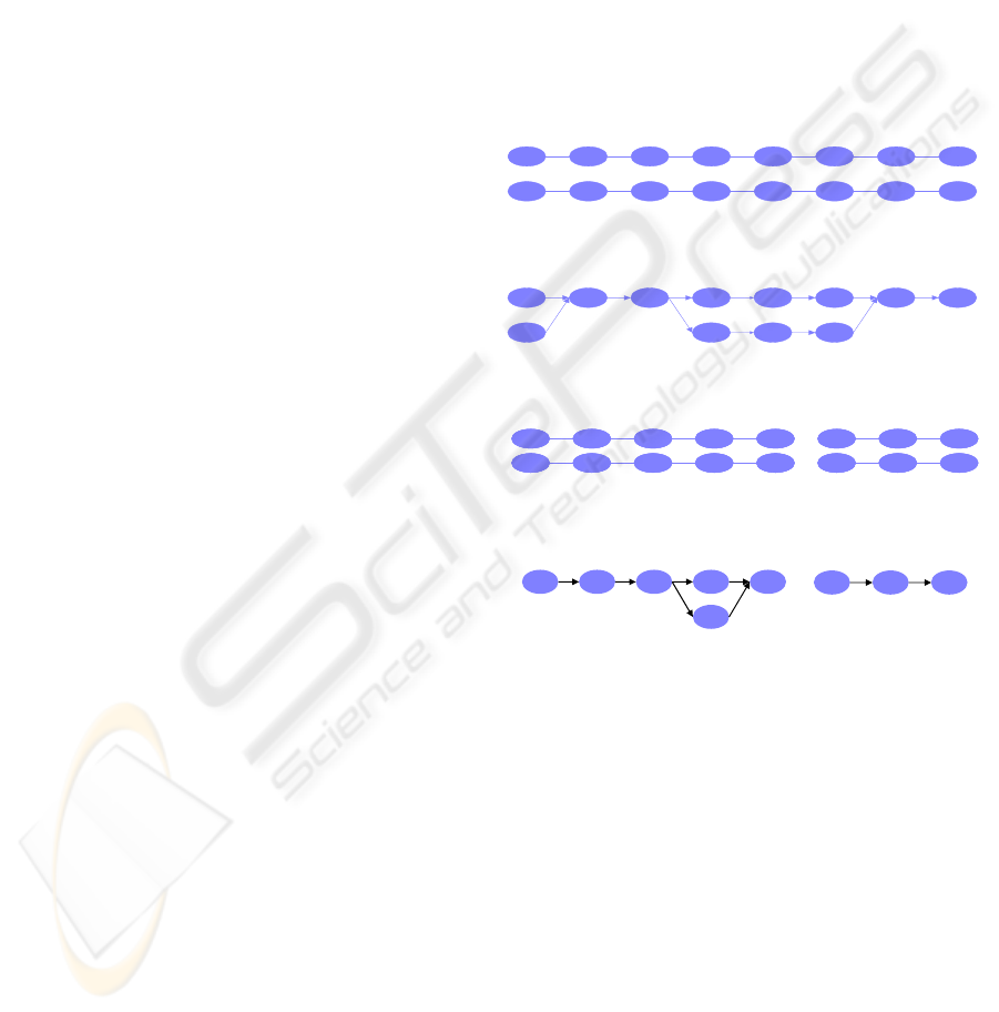
To illustrate the application of the extension of the
Stochastic Approach proposed in this paper, the algo-
rithms will be applied with the subsequences of two
different sequences of the Figure 2. Naturally, the
products (i.e. the wafers) follow the same series of
state with these two subsequences. The BJT4G algo-
rithm produces the model of Figure 3.
1095 1190 1274 1104 10521264
1095 1190 1275 1106 10521261
1043 1264
1041 1264
Figure 2: The Ω set of sequences ω
1
(up) and ω
2
(down).
1095 1190 1274 1104 10521264
1275 11061261
1043 1264
1041
Figure 3: Model made with the BJT4G algorithm with Ω.
6024 6043 6064 60586013
6024 6043 6065 60586013
6024 6043 6064 60586013
6024 6043 6065 60586013
6026 6015 6058
6026 6015 6058
6026 6015 6058
6026 6015 6058
Phase 1
Phase 2
Figure 4: Process Phases (ω
i
k
Subsequences).
6013 6024 6043 6064
6065
6058
6026 6015 6058
Phase 1
Phase 2
Figure 5: Model of each phase.
The equivalence classes created with the algo-
rithm 1 are singletons of the form C
i
= {(φ
i
, i)} with
i ∈ [6012, . . . , 6065]. For example, the class of equiv-
alence C
6013
= {(φ
6013
, 6013)} contains 15 classes:
C
6013
= { C
1031
, C
1032
, . . ., C
1045
}. This algorithm
rewrites the two subsequences of Ω (Figure 2) to pro-
duce the sub sequences of Figure 4. It is easy to
see that the equivalence class of the classes C
1043
and
C
1041
isC
6013
, when the equivalence class of theC
1095
is the C
6024
. With the rewritten sequences, the algo-
rithm 2 identifies the two process phases Ω
1
= { ω
1
1
,
ω
2
1
} and Ω
2
= { ω
1
2
, ω
2
2
} of Ω (Figure 4). The algo-
rithm 3 is then used with Ω = { Ω
1
, Ω
2
} to build the
models M
1
and M
2
of Figure 5. The process model
is simply provided with the union of the two models:
M = M
1
S
M
2
.
ICSOFT 2008 - International Conference on Software and Data Technologies
190

6033 6058
6027 6035
6047 6013 6024 6043
6064
6058 6026 6015
6058 6037 6058 6046 6050
6051 6013
6022
6064 6054
6042
6060
6050
6058 6045 6012 6058 6029 6043 6064
6058 6026 6012
6030 6043 6064
6053 6029
6050
6012 6030 6043 6064
[ 01:16:18 ,10j ]
[
13:58:17 ,1j 14:56:2 3 ]
[
02:49:30,23:20:16 ]
[
05:25:43 ,10:27:36 ]
[
01:26:07 ,1j 14:01:4 8 ]
[ 02:16:19 , 6j 14:02:56 ]
[
03:52:45, 7j 01:08:08 ][ 01:24:31 , 03:34:49 ]
[02:08:32, 11:29:1 8 ]
[07:56:41, 3 j 03:21:40 ]
[
02:01:4 1,04:52:13 ]
[
02:08:40 ,05:53:49 ]
[
01:44:19 ,1 j 08:12: 34 ]
[
01:55:14 , 16:55:3 0 ]
[
04:32:33 , 16:17:04 ]
[
01:25:58 , 15:52:56 ] [ 02:09:30 , 21:30:40 ] [ 02:08:10, 06:17:04 ][ 01:40:54 , 02:38::0 9 ] [ 01:32:4 0, 07:07::5 0 ] [ 03:03:04 , 4j 08:18 :44 ]
[
04:07:19 21:51:41 ]
[
06:13:42 20:53:45 ]
[
03:27:2 4 5j 07:23: 24 ] [ 10:35:29 10:35:29 ] [ 08:25:0 6 5j 13:53:2 9 ]
[
01:32:19 05:28:33 ] [ 01:43:45 05:17:57 ]
[
01:58:07 04:14:28 ]
[
09:18:02 4j 17:50:2 6 ]
[
02:35:05 2j 06:12:4 5 ]
[
04:48:1 9 18:40:12 ]
[
01:31:12 8j 04:32:2 4 ]
[
01:58:44 04:15:18 ]
[
013:23:4 02:22:48 ]
[
01:20:04 04:33:56 ] [ 02:54:50 3j 03:19:23 ][ 01:23:35 3j 21:37:11 ] [ 01:20:16 04:41:13 ]
[
02:52:1 0 2j 11:14 :12 ]
[
02:38:03 13j 09:26 :05 ]
[04:03:18 1j 01:22:36 ]
[04:18:34 2j 20:36:2 2 ]
[01:38:42 29j 02:26:17 ]
[07:43:27 11j 20:26:04 ] [04:54:36 20j 22:00:1 0 ]
….
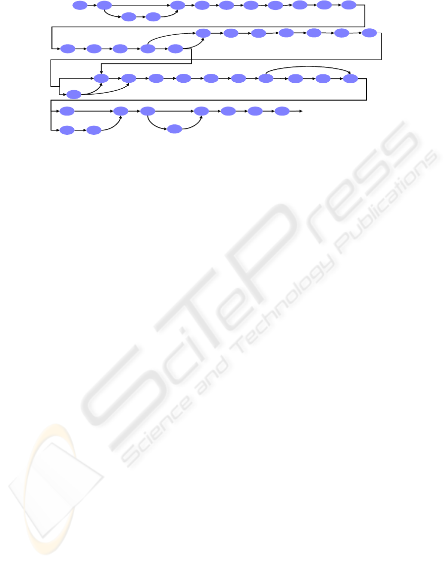
Figure 6: The first part of the process model.
Applied to the 45 sequences, the algorithm 4
builds a process model that contains 439 classes of
equivalence (i.e. nodes): this process model repre-
sents a wafer manufacturing road under the form of a
set of timed sequential binary relation between equip-
ments. The Figure 6 shows the beginning of this
model. Each of the 45 sequences is an instance of
this model. The STMicroelectronics experts are cur-
rently analyzing this model to validate the meaning of
a road represented at the equipment level of granular-
ity. This validation task is difficult because of the size
of process model.
5 CONCLUSIONS
This paper presents an extension of the Stochastic Ap-
proach framework to the modeling of manufacturing
processes from the timed data contained in the super-
vision system database. One of the interesting fea-
tures of the Stochastic Approach framework of mod-
eling is the notion of discrete event class. This no-
tion is used to define a process phase concept and
discrete event classes of equivalence that are required
large scale manufacturing processes. The definition
of these concepts leads to a global algorithm that has
been applied to the modeling of the electronics plates
manufacturing process of the Rousset plant of the
STMicroelectronics Company. This concrete appli-
cation shows the operational flavor of the extensions
of the Stochastic Approach Framework.
REFERENCES
Agrawal, R., Gunopulos, D., and Leymann, F. (1998). Min-
ing process models from workflow logs. In Sixth In-
ternational Conference on Extending Database Tech-
nology, pages 469–483.
Cook, E. J. and Wolf, A. L. (1998). Discovering models
of software processes from event-based data. ACM
Transactions on Software Engineering and Methodol-
ogy, 7:215–249.
Cook, E. J. and Wolf, A. L. (2004). Event-based detec-
tion of concurrency. In Proceedings of the 6th ACM
SIGSOFT international symposium on Foundations of
software engineering, volume 53, pages 35–45.
Ghallab, M. (1996). On chronicles: Representation, on-line
recognition and learning. Proc. Principles of Knowl-
edge Representation and Reasoning, Aiello, Doyle
and Shapiro (Eds.) Morgan-Kauffman, pages 597–
606.
Le Goc, M. (2006). Notion d’observation pour le diagnostic
des processus dynamiques: Application `a Sachem et
`a la d´ecouverte de connaissances temporelles. Hdr,
Facult´e des Sciences et Techniques de Saint J´erˆome.
Le Goc, M., Bouch´e, P., and Giambiasi, N. (2005). Stochas-
tic modeling of continuous time discrete event se-
quence for diagnosis. 16th International Workshop on
Principles of Diagnosis (DX’05) , California, USA.
Pinter, S. and Golani, M. (2004). Discovering workflow
models from activities’ lifespans. In Special issue:
Process/workflow mining, volume 53, pages 283–296.
Schimm, G. (2004). Mining exact models of concurrent
workflows. In Computers in Industry, volume 53(3),
pages 265–281.
van der Aalst, W., Weijters, T., and Maruster, L. (2004).
Workflow mining: Discovering process models from
event logs. In IEEE Transactions on Knowledge and
Data Engineering, volume 16, pages 1128–1142.
van der Aalst, W. M. P. and Weijters, A. J. M. M. (2004).
Process mining. Special issue of Computers in Indus-
try, 53:231–244.
Weijters, A. and van der Aalst, W. (2003). Rediscovering
workflow models from event-based data using little
thumb. In Integrated Computer-Aided Engineering,
volume 10(2), pages 151–162.
USING THE STOCHASTIC APPROACH FRAMEWORK TO MODEL LARGE SCALE MANUFACTURING
PROCESSES
191