LASER SIMULATION

Methods of Pulse Detection in Laser Simulation

Jana Hájková

Department of Computer Science and Engineering, University of West Bohemia, Univerzitní 22, Pilsen, Czech Republic

Keywords: Simulation, visualization, method, pulse detection, laser, application approach, automation, centre of mass.

Abstract: This paper deals with the problem of laser simulation. At the beginning it gives a broader overview of the

project of laser simulation which is processed at the University of West Bohemia. The simulation is

described in several fundamental steps, a technique of data obtaining, processing and usage for the

simulation is highlighted to understand the whole approach well. Three methods for automatic pulse

detection are described in detail. Pulse detection is the main part of the pulse extraction, which is one of the

most important data processing steps. The main idea of each described method is explained and their

problems and possible ways of their elimination are discussed. At the end of the paper future plans for the

project with the focus on the alternatives of system automation are introduced.

1 INTRODUCTION

About one year ago a project started in a cooperation

of several departments of University of West

Bohemia – the Department of Computer Science and

Engineering, the Department of Physics and the

Department of Cybernetics. Also the Department of

Mathematics from the same university is partly

interested in the project. Except these four university

departments, also a hi-tech company Lintech

participates in this project and supports it.

Our aim is to develop a real laser equipment

(HW device) for sophisticated laser burning into

various materials. Besides the excellent HW

components this device must have also several

indispensable SW modules, which control the laser,

simulate its function or enable to explore burned

experiments. The basics of the whole project and its

parts are detailed in (Hájková and Herout, 2008).

The task for our group is to create a SW support

in the form of simulation system for offline and

online controlled simulations and a sophisticated

tool for exploring of burned experiments which

could be used independently.

The paper is divided into six chapters. Following

Section 2 describes the basic simulation process, in

Section 3 methods for automatic pulse detection are

worked out and in Section 4 our results are outlined.

Section 5 presents out future plans and Section 6

concludes the paper.

2 LASER SIMULATION

The whole system of laser device should serve for

miscellaneous scientific and commercial

experiments. Results of these experiments are not

fully deterministic, that is why they sometimes need

to be reoperated several times to obtain optimal

result. Repetitious burning of the same experiment is

money and time consuming. That is why any

software tool which would eliminate real burning of

incorrect results is beneficial.

The simulation should provide experiments as

quick and cheap as possible. It would also enable

optimization from different points of view (e.g.

speed or accuracy) and help to eliminate the

unreasonable experiments. All parts of the

simulation should be automatic in the maximal way

so the simulation can run independently of the user.

Moreover, in contrast to real burning, where each

experiment requires servicing, simulation creates a

possibility of batch-oriented experiments executing.

After the simulation finishes, the best results can be

selected and all gained results are described.

As a part of the simulation there should be also

implemented a tool for data 2D and 3D

visualization. This tool would enable to explore real

or simulated results and to interpret accuracy and

optimality of the simulated sample.

Each simulation has to be based on the

simulation model. We decided to use an application

186

Hájková J. (2008).

LASER SIMULATION - Methods of Pulse Detection in Laser Simulation.

In Proceedings of the Third International Conference on Software and Data Technologies - SE/GSDCA/MUSE, pages 186-191

DOI: 10.5220/0001885001860191

 SciTePress

approach; it means that our simulation model comes

out from real data measured from real burned

experiment.

2.1 Data Description

At first, the way of data obtaining should be

described. To get any data for the simulation input,

samples have to be burned by existing laser

equipment into the real material. After burning the

real samples, they have to be measured. For this

purpose the confocal microscope Olympus LEXT

OLS3100 is used.

The sample surface is represented by the matrix

of floats expressing heights in corner points of the

uniform rectangular grid. This grid represents a

height map which describes the surface of the

sample.

The majority of samples which we use have the

same form. The burned pulse fills preponderance of

the sample surface; the real dimension of the sample

is 256×192μm. The grid of height map is really fine;

most common grid step in used data is 0.25μm. It

means that the surface of such sample is described

by 1024×768 values. We dispose with samples

burned into two materials: steel and cermet (a

composite material composed of ceramic and

metallic materials).

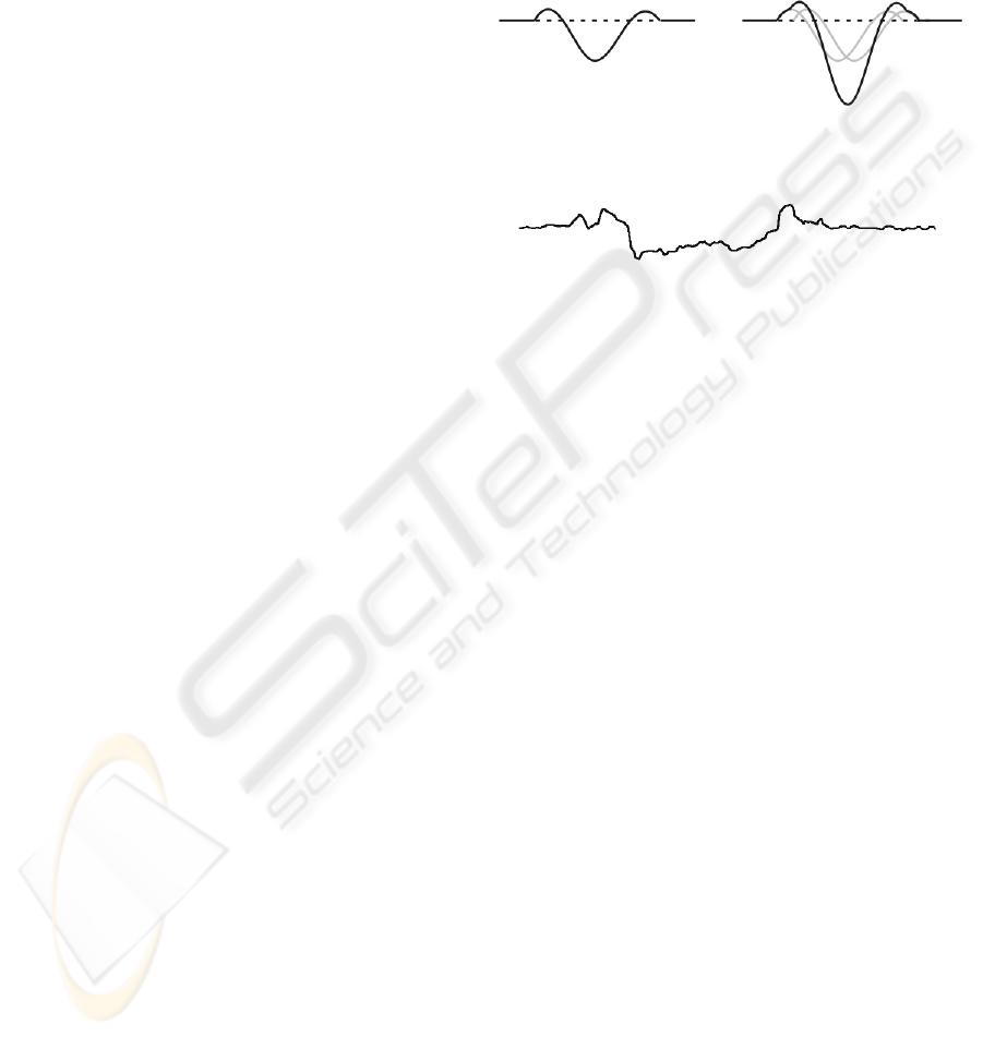
2.1.1 Pulse Representation

Let’s explore the pulse in a detail, at first with a little

bit simplification. In an ideal situation the surface of

the material would be perfectly smooth without any

roughness. When the laser burns one pulse into such

material, it will modify the surface, a hollow in the

point of burning will be created and around the

hollow the melted material will make a bulge (as

seen in

Figure 1a). By these conditions if we place

two laser pulses at almost one place, we can use a

principle of summation. Result is shown in the

Figure 1b where two pulses next to each other are

placed.

But in the real environment we can hardly expect

ideal conditions. Because we use real data which are

measured with high zoom, roughness of the material

plays quite important role and the surface roughness

causes inconsiderable problems during the sample

processing. Cross-sections of real pulse (1 pulse

burned into the cermet) can be seen in

Figure 2.

At the beginning of our work it was important to

choose any suitable form of pulse representation. At

first we planned to represent the pulse by several

parameters or by its cross-section. The whole pulse

should be gained as a surface of revolution. It means

that the surface of the sample would be obtained by

rotating the curve of cross-section in space about an

axis passing throw the middle. This method could be

used in the case of ideal situation, but in the case of

real samples this representation of the pulse would

mean unacceptable distortion of data.

a) b)

Figure 1: Simplified result of burning into ideally smooth

material a) one pulse b) two pulses next to each other.

Figure 2: Cross-section of real pulse.

That is why we had to search for another way of

pulse representation. Finally we decided for the form

of height map representation of the whole pulse

surface. There was a question how to describe the

values of the pulse surface to be used for the burning

simulation in the simplest way. From several

experiments we decided to represent the level of the

material by the value of zero. All points of the

sample height map are during pulse extraction

recounted and saved as differences of the surface of

the material and their original height. It means that

the final saved pulse consists of positive and

negative real values. The positive values represent

material upon the basic material level; on the

contrary the negative ones represent material which

has vaporized.

The format of height map is exact enough, but its

disadvantage embodies in amount of data files which

have to be saved for various pulses for different

materials. The size of the file is not very high but we

still speculate about the redundancy of this format.

That is why we would like to try another method of

pulse representation.

Pulses are extracted from input samples. Because

of high amount of input samples it is necessary to

make the process of pulse extraction automatic. The

main part of the process is created by the automatic

pulse detection. Because it is the main topic of this

paper, it is particularized separately in Section 3.

LASER SIMULATION - Methods of Pulse Detection in Laser Simulation

187

2.2 Simulation Approach

As it was described in (Hájková and Herout, 2008),

we decided to use for the simulation the application

approach.

The pulses are extracted from input data for

given combination of used material and laser setting.

The basic technique of simulation of samples

burning is to place selected pulses gained from input

data on the surface of the unburned material. The

format of the pulse is designed for the simplest

usage as possible and it offers the ability of direct

pulse application on the surface of the material (as it

was described in the previous sections).

The simulation itself requires solving of many

problems (e.g. heating of the material during

repetitive burning of laser ray into one point of the

material, influence of the material surface roughness

on the laser ray reflection or inaccuracies caused by

starting and finishing laser motion).

For the correct function of the simulation the

system has to be verified. During the verification the

burned samples are compared with the real ones,

which are gained by the same method as it was

described in Section 2.1. To test and evaluate the

system in a more global way a broad range of

samples has to be simulated and compared. An

automatic verification is used for speeding it up.

3 METHODS FOR AUTOMATIC

PULSE DETECTION

Pulse detection is used as a part of data

preprocessing. The task of detection is to define the

area of the material surface which was affected by

the laser burning as exactly as possible. Pulse

detection can be done of course manually but for the

speedup and simplification of the whole preparation

process, the system has to prepare maximum of parts

self-containedly. But the precision and accuracy has

to be preserved as well with the automation process.

That is why we have to develop appropriate

algorithm for pulse detection.

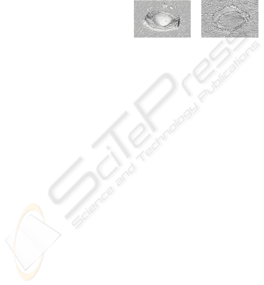
The main problem is the roughness of the basic

material surface. As it can be seen in

Figure 3 for

some materials, such as for a steel in

Figure 3a, the

surface is quite smooth. Another situation comes in

the case of cermet (

Figure 3b), where the protrusions

on the material surface are more noticeable.

Moreover, for all types of material also local

roughnesses which are not specific for the material

can appear. Such defects need not to be visible on

the material surface by naked eye, but thanks to the

height resolution of real sample scanning, they are

included in the description of the sample and are the

source of problems during the pulse auto-detection.

Local roughness can be seen in

Figure 3a on the

upper side of the sample.

a) b)

Figure 3: a) Surface of steel with relatively smooth

surface; local defect can be seen on the upper side of the

sample. b) Surface of cermet sample with globally higher

roughness of the surface.

The user is able to distinguish roughness or

defects of the material during the manual pulse

detection, but for the automatic method it is very

difficult to differentiate these inaccuracies from the

border of the pulse. Chosen methods have to be

precise enough, but very precise methods are already

slow. Quickly working methods are unfortunately

inaccurate. That is why we have to find a

compromise and to create a new method designed

right for this task.

3.1 Global Extremes Method

The first version of detection algorithm goes from

unmodified sample surface. The algorithm starts

from points with the minimal and maximal height.

These points are supposed to be in the area of the

burned pulse that should be detected. From their

position columns of height map to the left and to the

right side are inspected and the height difference of

points in each single column (it means the difference

between the maximal and minimal value in the

column) is counted. If the value does not exceed

given height limit, an inspection in the direction is

finished. After cutting of columns on the left and

right side of the pulse, the same process of border

searching is started for rows. Horizontal borders are

appointed.

There is a question how to gain the value of

difference height limit. This is one of problems of

this algorithm. If we do not want to set the constant

manually we have to explore the sample

automatically, for example during its loading into

the system. We can suppose that borders of the

sample are not modified by the burning and that is

why they represent the original material surface and

ICSOFT 2008 - International Conference on Software and Data Technologies

188

so the difference constant can be for most samples

precounted, for example as the minimal height

difference counted from several border columns. But

this approach may not work well if the used border

of the sample is damaged by any local defect of the

material. In such case the difference constants is

counted too high.

The worse problem that causes wrong results of

this method is brought by local defects of large

height or depth. The defect can move the location of

global minimum or maximum from the area of the

pulse to the area of local defect. This problem can be

solved by changing of the algorithm for the starting

point searching.

3.2 Centre of Mass Method

Another way how to get the starting point for

automatic pulse detection is to find the position of

centre of mass in the sample. The typical procedure

of the center of mass computation has to be adapted

for the sample representation. Basic expression for

calculation of the center of mass x

of a system of

particles is defined as the average of the particle

positions x

, weighted by their masses m

(1).

∑

(1)

Let us label the point of the sample as f

= f[x, y].

Because the whole sample is represented by positive

values (the values representing the material level in

the sample are given by the height of the material

into which the sample was burned), we could define

= f

. The simplified cross-section curve of the

sample can be seen in

Figure 4a. The result is shown

Figure 5a. If the pulse does not take the majority

space of the sample and the pulse is not placed in the

centre of the sample, the rest of the surface

overbalances the pulse area and the centre of mass is

moved from the centre of the pulse partly to the side

of plain surface.

That is why it is necessary to shift the whole

sample so that the material level is represented as a

zero value. By this shifting some parts of the sample

are represented by the negative value. Such sample

cannot be used for center of mass computation and

so the negative values have to be converted to

positive ones. That can be done by using power

function with even and positive exponent. To stress

values of the pulse from small values in the

neighbourhood of the zero level, we decided to use

exponent 4 (

Figure 4b). Finally the weights for center

of mass computation are defined as in the expression

(2), where basicLevel represents the height of the

basic material. The result of such calculation can be

seen in

Figure 5b.

(

)

basicLevelfm

−=

(2)

a) b)

Figure 4: Simplified cross-section of the sample in all both

phases of computation; a) the original sample, b) the

sample after application of power function.

a) b)

Figure 5: a) The result of the centre of mass computation

with the weight m

= f

. b) The result of the centre of mass

computation with the weight m

= (f

-basicLevel)

By this method we get the starting position

which is placed in the area of burned pulse and is

affected by local material defect in a minimal way.

The other steps of algorithm described in Section 3.1

can be used in this time or we can choose another

technique which is described in Section 3.3.

3.3 Spiral Method

During testing the location of starting point was

always found correctly in the area of burned pulse

for all samples we dispose with. So we can try to use

another approach for finding borders of the pulse

(previously described algorithm of pulse borders

detection is sensitive to local defects on the material

surface). We can start in the starting point and then

inspect the surroundings up to finding the basic level

of the material.

In the ideal case, the pulse has circular or

ellipsoidal shape and the centre of mass is placed

exactly in the centre of the pulse. For such pulse we

can find the bounding rectangle simply. If we put

through the centre of mass two lines parallel with

axis x and y (as can be seen in

Figure 6a), we can

make cross-sections of the sample along these lines

(the vertical and the horizontal ones).

The cross-section curve is optimally in the area

of the pulse more diverted than in the part of the

LASER SIMULATION - Methods of Pulse Detection in Laser Simulation

189

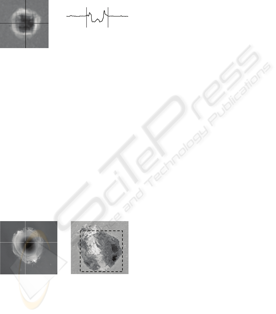
unburned material. That is why we can determine

two points of the curve, where the pulse finishes and

to define borders there (

Figure 6b).

a) b)

Figure 6: a) Sample with nearly circular shape; two lines

parallel with axis x and y are going through the centre of

mass. b) Cross-section curve with defined borders.

Searching of border values starts at the beginning

and at the end of the curve and continues in the

direction to the centre of mass. First, we are in the

area of unburned material where values of the curve

do not differ from the average material height a lot.

When the values start to differ more we have found

the border of the pulse. To prevent mistakes caused

by roughness of the material, the same height limit,

as in the algorithm described in Section 3.1 (gained

during the sample loading), is used.

In the real cases the method described above is

not sufficient, but we can use its result as a starting

state for the next processing. If the shape of the

pulse is irregular, the centre of mass is shifted from

the middle of the pulse (as in

Figure 7a). Moreover,

the irregularity of the pulse from the top view

deflects the borders (as in

Figure 7b). That is why the

previous procedure gives only a rectangle that

borders a part of the pulse.

a) b)

Figure 7: a) Shifted position of the centre of mass location.

b) Asymmetry of the pulse shape in the top part of the

pulse from the top view that will cause top border shifting.

The border determined by the algorithm is dashed.

The final borders are searched in a spiral way.

All borders are periodically tested if it is possible to

move them for one row or one column further from

the centre of mass. In each step for each single

border (left, bottom, right and top) the height

difference between the minimal and the maximal

value in the shifted position is computed and

compared with the difference limit for the processed

sample. The sequence of borders is preserved

through the whole computation (it means borders are

rotating during the algorithm). If any border can not

be moved it is not used any more in following steps.

4 RESULTS

To describe all results of existing SW part of the

project, a highly specialized tool which was

designed and subsequently also implemented would

have to be mentioned, because there was no

available tool for data exploring and modification.

Because this paper is focused on the topic of

automatic pulse detection methods so this section

will concentrate only on results of these methods.

Several methods for pulse detection were

described. All methods were tested on the same

samples which were chosen because of any typical

feature. The task of the algorithm has been to detect

the pulse in the most perfect way. In this section

problematical samples are described and discussed.

Some of tested samples are burned into cermet,

where the high roughness of the material can

influence the detection and some are burned into

steel which has much smoother surface. Samples

with various counts of laser pulses burned into one

point of the material were chosen. Surfaces of

several samples are influenced by the local defects

of the material and shapes of pulses are in some

cases more and in some less asymmetric.

A feature which is problematical for all methods

is the determination of height difference limit. The

way of precounting the value as the minimal height

difference counted from several border columns

works quite well for the samples without local defect

on the material surface. But the areal defect around

the pulse can produce incorrect pulse detection as it

is shown in

Figure 9a.

Another problem is the roughness of the material

surface for example in the case of cermet. Each of

methods copes with it in a little bit different way.

Results of the Centre of mass method are shown in

Figure 8a and it can be compared with the result of

the Spiral method in Figure 8b. The value of height

difference limit was computed too high because of

the roughness of the material. In the first case where

left and right border were found first, part of the

pulse was not bordered. In the second case, thanks to

the spiral approach, this did not happen at the cost of

expansion of bordering rectangle.

ICSOFT 2008 - International Conference on Software and Data Technologies

190

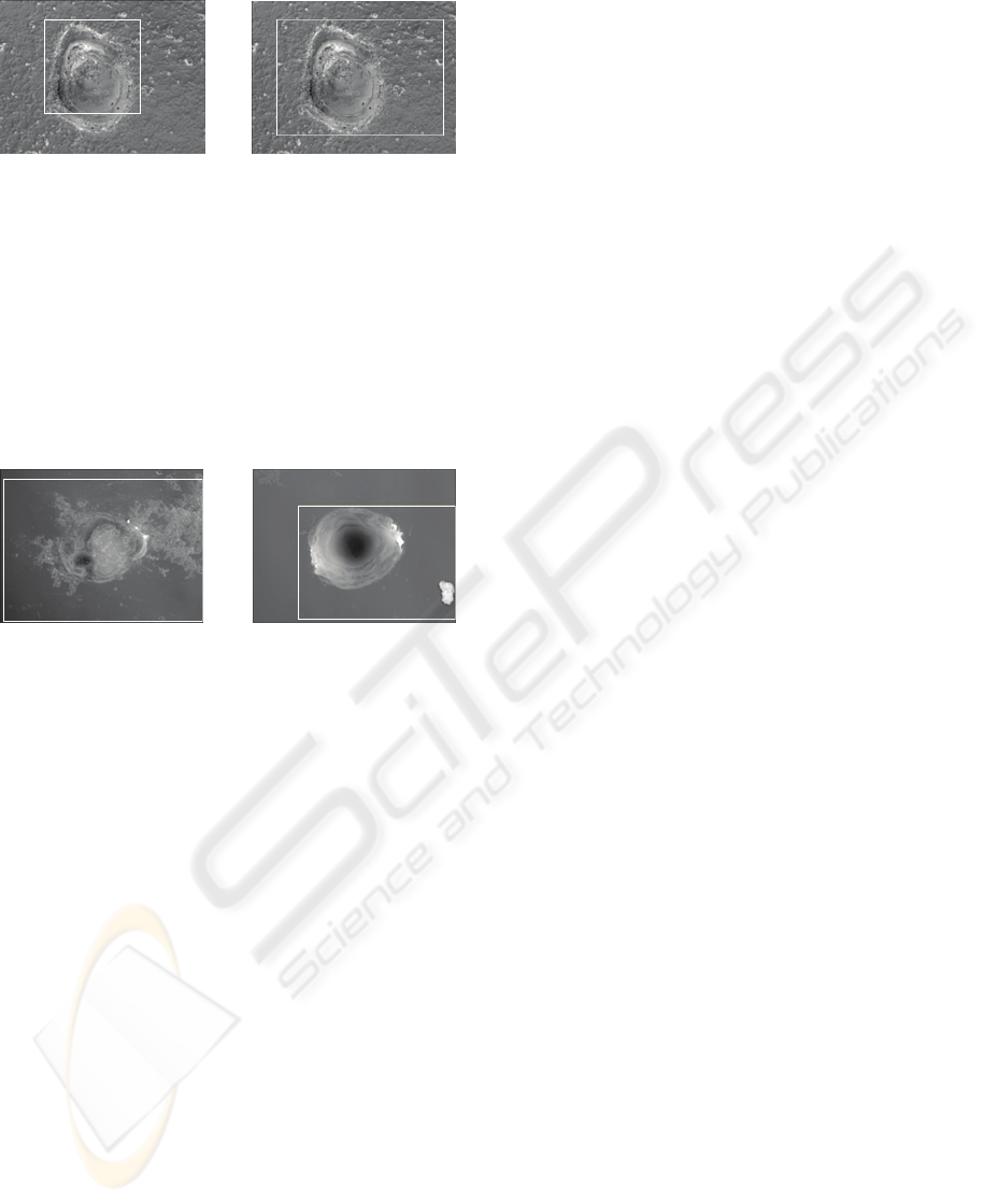
a) b)

Figure 8: Comparison of pulse detection in the sample

with high roughness of the material – a) Centre of mass

method; b) Spiral method.

The main disadvantage of the method starting

from global extremes is in the setting of the starting

position. If there is any local defect of extreme

height, the starting point for pulse border searching

is shifted into the position of local defect and the

result is distorted. The sample corresponding to such

situation can be seen in

Figure 9b.

a) b)

Figure 9: Problematic samples with local defects a) of

areal character around the pulse which causes incorrect

pulse detection; b) of extreme height in the surrounding of

the sample which causes wrong localization of starting

position.

5 FUTURE PLANS

Our future plans are divided into several groups in

dependence to which activity it is related to. Of

course, one of our most important aims is to improve

the simulation to get as realistic results as possible.

But with regards to the main topic of this paper let

us focus on our plans concerning improvements of

program self-activity.

The whole system should work as automatic as

possible. That is why all partial tasks of data

processing should be self-acting if possible. Of

course, despite the automation, the reliability and

speed of the system must be preserved.

All methods for pulse detection described above

use similar principles and that is why they face the

similar problems. So we decided to try to test

another approaches. One of the tested alternatives

are methods used for image processing and

recognition such as thresholding, erosion, dilatation,

edge detection, pattern recognition, various types of

image filtration etc. (Hlaváč and Šoula), (Hlaváč and

Sedláček). These methods are in the process of

testing for the present and they are not used for the

detection itself yet. Methods are tested in

combination with different variants of resampling of

the image. The results look well so far, the main

problem is the automaticity of the detection process,

because for each sample the setting is different.

Another way to automatic pulse detection might

be methods using linear and non-linear diffusion

filtering (Nishiguchi, Imiya and Sakai) in the

combination with isolines searching. Also this

approach is in the phase of testing.

6 CONCLUSIONS

The project is in the phase of partial completion. We

have prepared a tool for data preprocessing and

groundwork for simulation tool. It enables us to

provide various experiments. For this purpose we

dispose with data sets from experiments burned and

measured for two materials – cermet and steel.

In the close future we plan to maximize the

self-activity of the pulse detection tool and we want

to improve methods for system verification and

results comparison.

ACKNOWLEDGEMENTS

The work was supported by the Ministry of

Education, Youth and Sport of the Czech Republic

“University spec. research – 1311”.

REFERENCES

Blelloch, E. G., 2001. Introduction to Data Compression

[online], [cit. 2008-03-28].

<http://www.cs.cmu.edu/afs/cs/project/pscico-

guyb/realworld/www/compression.pdf>

Hájková, J., Herout P., 2008. Laser Simulation.

Proceedings of the 7th International Conference

APLIMAT 2008, STU Bratislava.

Hlaváč, V., Šoula, M., 1994. Image Processing and

Machine Vision, Chapman & Hall Computing,

London.

Hlaváč, V., Sedláček, M., 2001. Zpracování signálů a

obrazů, Vydavatelství ČVUT. Praha.

Nishiguchi, H., Imiya, A., Sakai, T., 2006. Laplacian

Based Non-Linear Diffusion Filtering. Proceedings of

18th International Conference on Pattern Recognition

ICPR 2006.

LASER SIMULATION - Methods of Pulse Detection in Laser Simulation

191