ASSESSMENT OF THE EFFECT OF NOISE ON AN UNSUPERVISED

FEATURE SELECTION METHOD FOR GENERATIVE

TOPOGRAPHIC MAPPING

Alfredo Vellido and Jorge S. Velazco

Department of Computing Languages and Systems (LSI), Technical University of Catalonia (UPC), Barcelona, Spain

Keywords:

Unsupervised Feature Selection, Feature Relevance Determination, Generative Topographic Mapping, clus-

tering, uninformative noise.

Abstract:

Unsupervised feature relevance determination and feature selection for dimensionality reduction are important

issues in many clustering problems. An unsupervised feature selection method for general Finite Mixture

Models was recently proposed and subsequently extended to Generative Topographic Mapping (GTM), a

nonlinear manifold learning constrained mixture model for data clustering and visualization. Some of the

results of a previous preliminary assessment of this method for GTM suggested that its performance may be

affected by the presence of uninformative noise in the dataset. In this brief study, we test in some detail such

limitation of the method.

1 INTRODUCTION

Statistical Machine Learning (SML) provides a uni-

ﬁed principled framework for machine learning meth-

ods and helps to overcome some of their limitations.

Embedding probability theory into machine learning

techniques has important modeling implications. For

instance, it requires modeling assumptions, includ-

ing the speciﬁcation of prior distributions, to be made

explicit; it also automatically satisﬁes the likelihood

principle and provides a natural framework to handle

uncertainty.

An example of SML can be found in Finite Mix-

ture Models (FMM), which are ﬂexible and robust

methods for multivariate data clustering (McLachlan

and Peel, 1998). The addition of visualization capa-

bilities would beneﬁt these models in many applica-

tion scenarios, helping to provide intuitive cues about

data structural patterns. One way to endowFMM with

data visualization is by constraining the mixture com-

ponents to be centered in a low-dimensional manifold

embedded into the multivariate data space, as in Gen-

erative Topographic Mapping (GTM) (Bishop et al.,

1999). This is a non-linear, neural network-inspired

manifold learning model for simultaneous data clus-

tering and visualization.

The interpretability of the clustering results pro-

vided by GTM becomes difﬁcult when the analyzed

data sets consist of a large number of features. This

limitation can be overcome with methods to estimate

the ranking of the data features according to their rel-

ative relevance, leading to feature selection (FS). The

research on unsupervised FS is scarce in comparison

to that for supervised models, despite the fact that FS

becomes a paramount issue in many clustering prob-

lems. A description of the problem in terms of a re-

duced subset of relevant features would improve the

interpretability of the clusters obtained by unsuper-

vised methods.

An important advance on unsupervised FS for Fi-

nite Mixture Models was presented in (Law et al.,

2004) and recently extended to GTM (the FRD-GTM

model) in (Vellido et al., 2006) and to one of its vari-

ants for time series analysis (FRD-GTM-TT) in (Olier

and Vellido, 2006). This method was preliminarily

assessed in (Vellido, 2006), where some of the re-

sults suggested that the performance of the method

may be degraded by the presence of uninformative

noise, which would obscure the underlying cluster

structure of the data and, therefore, mislead an unsu-

pervised feature relevance estimation method. In this

brief study, we provide evidence of the limitations of

the method through controlled experiments using syn-

thetic data.

The remaining of the paper is organized as fol-

lows. First, brief introductions to the standard Gaus-

sian GTM and its extensionfor Feature Relevance De-

termination (FRD) are provided in section 2. This is

424

Vellido A. and S. Velazco J. (2008).

ASSESSMENT OF THE EFFECT OF NOISE ON AN UNSUPERVISED FEATURE SELECTION METHOD FOR GENERATIVE TOPOGRAPHIC

MAPPING.

In Proceedings of the Tenth International Conference on Enterprise Information Systems - AIDSS, pages 424-430

DOI: 10.5220/0001681204240430

 SciTePress

followed, in section 3, by a description of the exper-

imental settings and, in section 4, by a presentation

and discussion of the results. The paper closes with a

brief summary of conclusions.

2 FEATURE RELEVANCE

DETERMINATION FOR GTM

2.1 The Standard GTM Model

The neural network-inspired GTM is a manifold

learning model with sound foundations in probabil-

ity theory. It performs simultaneous clustering and

visualization of the observed data through a nonlin-

ear and topology-preserving mapping from a visual-

ization latent space in ℜ

(with L being usually 1

or 2 for visualization purposes) onto a manifold em-

bedded in the ℜ

space, where the observed data re-

side. For each feature d, the functional form of this

mapping is the generalized linear regression model

(u,W) =

∑

(u)w

, where φ

is one of M ba-

sis functions, deﬁned here as spherically symmetric

Gaussians, generating the non-linear mapping from a

latent vector u to the manifold in ℜ

. The matrix W

of adaptive weights w

explicitely deﬁnes this map-

ping.

The prior distribution of u in latent space is con-

strained to form a uniform discrete grid of K centres.

A density model in data space is therefore generated

for each componentk of the mixture, which, assuming

that the observed data set X is constituted by N inde-

pendent, identically distributed (i.i.d.) data points x

leads to the deﬁnition of a complete log-likelihood in

the form:

L(W,β|X)=

∑

n=1



∑

k=1



2π



D/2

exp

{

−β/2ky

−x

}



(1)

where y

is a reference or prototype vector consisting

of elements (y

∑

), which are an in-

stantiation of the generalized linear regression model

described above. From Eq. (1), the adaptive param-

eters of the model, which are W and the common

inverse variance of the Gaussian components, β, can

be optimized by maximum likelihood (ML) using the

Expectation-Maximization (EM) algorithm. Details

can be found in (Bishop et al., 1999).

2.2 The FRD-GTM

In this paper, unsupervised feature relevance is under-

stood as the likelihood of a feature being responsible

for generating the data cluster structure. Therefore,

relevant features will be those which better separate

the natural clusters in which the data are structured.

Moreover, we are interested in unsupervised feature

selection methods that are suitable for clustering mod-

els that also provide data visualization. With that in

mind, the FRD technique was deﬁned for the GTM

model in (Vellido et al., 2006). For the unsupervised

GTM clustering model, relevance is deﬁned through

the concept of saliency.

The FRD problem was investigated for GTM in

(Vellido et al., 2006). Feature relevance in this unsu-

pervised setting is understood as the likelihood of a

feature being responsible for generating the data clus-

ter structure and it is quantiﬁed through the concept

of saliency. Formally, the saliency of feature d can

be deﬁned as ρ

= P(η

= 1), where η=(η

,... ,η

)

is a set of binary indicators that can be integrated in

the EM algorithm as missing variables. A value of

= 1 (ρ

= 1) indicates that feature d has the maxi-

mum possible relevance. According to this deﬁnition,

the FRD-GTM mixture density can be written as:

p(x|W,β,w

,β

,ρ)=

∑

k=1

∏

d=1

{

p(x

,β)+(1−ρ

(

0,d

,β

0,d

)}

(2)

where w

is the vector of W corresponding to fea-

ture d and ρ ≡ {ρ

,... ,ρ

}. A feature d will be

considered irrelevant, with irrelevance (1 −ρ

), if

p(x

,β) = q(x

0,d

,β

0,d

) for all the mix-

ture components k, where q is a common density

followed by feature d. Notice that this is like say-

ing that the distribution for feature d does not fol-

low the cluster structure deﬁned by the model. This

common component requires the deﬁnition of two ex-

tra adaptive parameters: w

≡ {w

,1,.. .,w

0,D

} and

≡ {β

0,1

,... ,β

0,D

} (so that y

= φ

). For

fully relevant (ρ

→ 1) features, the common compo-

nent variance vanishes:(β

0,d

)

−1

→ 0. The parameters

of the model can, once again, be optimized by ML

using the EM algorithm. Detailed calculations can be

found in (Vellido, 2005).

3 EXPERIMENTAL SETTINGS

The results of statistically principled models for prob-

ability density estimation, such as GTM and its vari-

ants, are bound to be affected, in one way or another,

by the presence of uninformative noise in the data.

Here, we assess such effects on the FRD-GTM model

described in the previous section. For that, data with

very speciﬁc characteristics are required. We use syn-

thetic sets similar to those in (Law et al., 2004) for

comparative purposes.

ASSESSMENT OF THE EFFECT OF NOISE ON AN UNSUPERVISED FEATURE SELECTION METHOD FOR

GENERATIVE TOPOGRAPHIC MAPPING

425

The ﬁrst synthetic set (hereafter referred to as

synth1) is a variation on the Trunk data set used in

(Law et al., 2004)), and was designed for its 10 fea-

tures to be in decreasing order of relevance. It con-

sists of data sampled from two Gaussians N (µ

,I) and

N (µ

,I), where



= 1,

√

,... ,

√

2d−1

,... ,

√



and µ

= −µ

. We hypothesize (H1) that the feature

relevance ranking estimated by FRD-GTM for these

data will deteriorate gradually as noise is added to the

10 original features and in proportion to its level. In

order to test H1, four increasing levels of Gaussian

noise, of standard deviations 0.1, 0.2, 0.5, and 1, were

added to the 10 original features of synth1, for a given

sample size. It is also hypothesized (H2) that the fea-

ture relevance ranking will deteriorate as we add new

noisy features and in proportion to their level of noise.

In order to test H2, 5 and 10 dummy features consist-

ing of Gaussian noise of standard deviations 0.1, 0.2,

0.5, and 1, were, in turn, added to the 10 original fea-

tures.

The second dataset (hereafter referred to as

synth2) consists of two features deﬁning four neatly

separated Gaussian clusters with centres located at

(0,3),(1, 9),(6,4) and (7, 10); they are meant to be

relatively relevant in contrast to any added noise. In

a ﬁrst experiment, noise of different levels was added

to the ﬁrst two features, while 4 extra noise features

were added to those two. Several other experiments,

similar to the ones devised for synth1 were designed

to further test H2.

The FRD-GTM parameters W and w

were ini-

tialized with small random values sampled from a

normal distribution. Saliencies were initialized at

= 0.5,∀d,d = 1,. . .,D. The grid of GTM latent

centres was ﬁxed to a square layout of 3 ×3 nodes

(i.e., 9 constrained mixture components). The cor-

responding grid of basis functions φ

was ﬁxed to a

2×2 layout.

4 EXPERIMENTAL RESULTS

AND DISCUSSION

The experiments outlined in the previous section aim

to assess the effect of the presence of uninformative

noise on the performance of FRD-GTM in the process

of unsupervised feature relevance estimation.

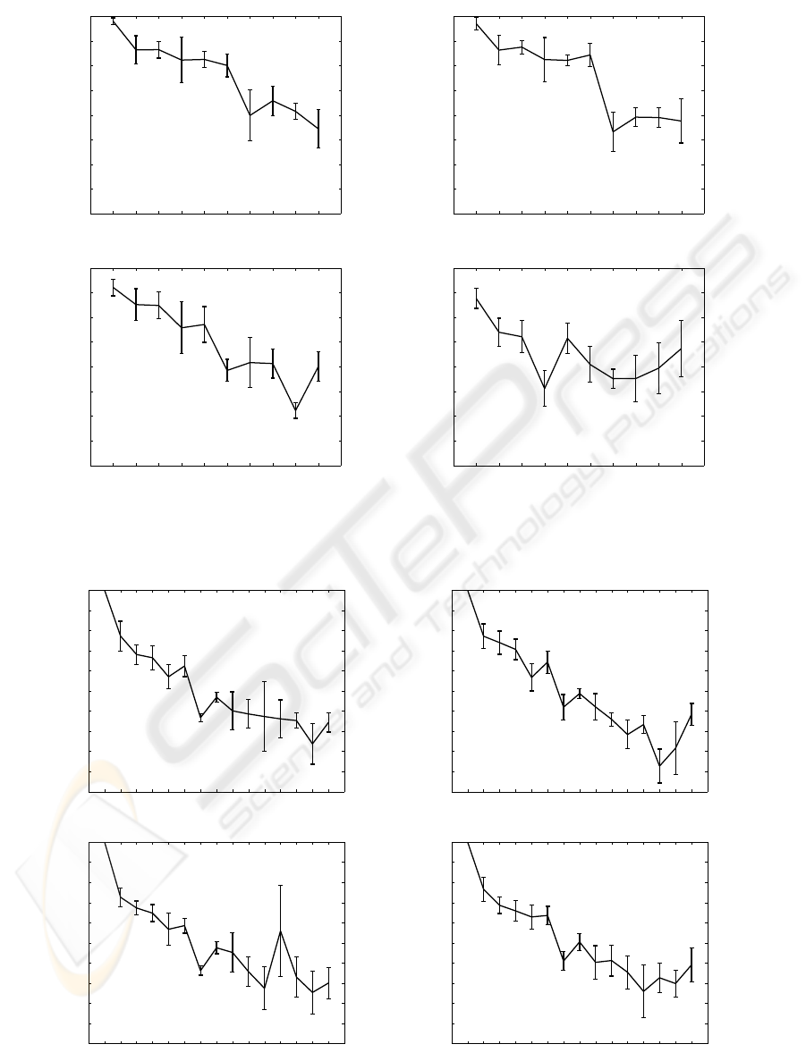
In the experiments reported in Figure 1, four lev-

els of Gaussian noise of increasing level were added

to a sample of 1,000 points of synth1. The FRD-GTM

is shown to behave robustly even in the presence of a

substantial amount of noise, although its performance

deteriorates signiﬁcantly for noise of standard devi-

ation = 1, as reﬂected in the breach of the expected

monotonic decrease of the mean feature saliencies. It

is also true that, comparing these results with those in

Figure 2 (in which no noise was added to synth1), the

most relevant feature is not so close to a saliency of 1.

H1 is, therefore, partially supported by these results.

The FRD ranking results for the second experi-

ment, using the 10 original features of synth1 plus 5

Gaussian noise features, are shown in Figure 2. For

all levels of noise, the relevance (in the form of esti-

mated saliency) of the original features (1 → 10) is

reasonably well estimated: the saliency for the ﬁrst

feature is close to 1 with almost full certainty (very

small vertical bars) and, overall, the expected mono-

tonic decrease of the mean feature saliencies is pre-

served, although breaches of such monotonicity can

also be observed. The saliencies estimated for the 5

added Gaussian noise features are regularly estimated

to be small. Interestingly, the increase in the level of

noise does not seem to affect the performance of the

FRD method in any signiﬁcant way: the differences

between the saliencies of the 10 original variables and

the 5 noisy ones stay roughly the same and the de-

creasing relevance for the 10 original variables does

not vary substantially. According to these results, H2

is not supported at this stage.

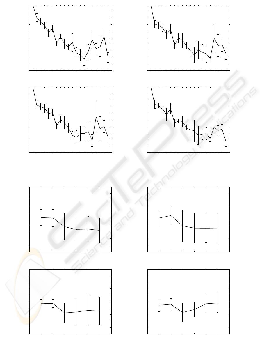
The FRD ranking results for the third experiment,

using the 10 original features of synth1 plus 10 Gaus-

sian noise features are shown in Figure 3. Once again,

and for all levels of noise, the relevance of the 10 orig-

inal features shows, overall, the expected monotonic

decrease of the mean feature saliencies, with some

breaches of monotonicity. This time, the saliencies

estimated for the 10 added Gaussian noise features

are not that clearly small in comparison to those esti-

mated for the 10 original ones. In summary, the de-

creasing relevance for the 10 original variables does

not vary substantially, and the differences between

the saliencies of the 10 original features and the 5

noisy ones stay roughly the same regardless the noise

level. Nevertheless, the FRD method seems to be af-

fected by the increase in number of the noisy features.

According to these results, H2 is only partially sup-

ported.

The FRD-GTM is shown to behave with reason-

able robustness when noise is added to the ﬁrst two

features of synth2, as shown in Figure 4. As in the

case of synth1, its performance deteriorates signiﬁ-

cantly for high levels of noise. Comparing these re-

sults with those in Figures 5 and 6 (in which no noise

was added to the ﬁrst two features), the overall dete-

rioration becomes evident. H1 is again partially sup-

ported by these results.

The FRD ranking results for the experiments us-

ICEIS 2008 - International Conference on Enterprise Information Systems

426

ing the 2 original features of synth2 plus either 7 or 10

Gaussian noise features are shown, in turn, in Figures

5 and 6. This is clearly a far easier problem for the

FRD method. Regardless the level of noise and the

number of added noisy features, FRD-GTM consis-

tently estimates the ﬁrst 2 features to be the most rele-

vant. Furthermore, the differences between the salien-

cies estimated for the ﬁrst 2 features and the added

(7 or 10) noisy ones stay roughly the same. In con-

trast with the results obtained in the experiments with

synth1, the estimated saliencies for all noisy features

are low and quite similar. Our research hypothesis H2

is not supported by these results.

5 CONCLUSIONS

In this paper, the effects of the presence of noise on a

method of unsupervised feature relevance determina-

tion for the manifold learning GTM model, have been

investigated in some detail.

The FRD-GTM has been shown to behave with

reasonable robustness even in the presence of a fair

amount of noise. It was ﬁrst hypothesized that the

feature relevance ranking would deteriorate as we add

noise to the existing features and in proportion to the

level of that noise. This hypothesis has found only

limited experimental support. It was also hypothe-

sized that the feature relevance ranking would dete-

riorate as we add extra noisy features to the existing

ones and in proportion to their number and the level

of noise. This second hypothesis has found little ex-

perimental support: There is only some evidence that

the performance of the FRD method deteriorates as

we increase the number of purely noisy features and

only if the dataset is complex enough.

This relative weakness of the method in the pres-

ence of noise makes it convenient to consider possi-

ble strategies for model regularization and, therefore,

future research will be devoted the design of meth-

ods for automatic and proactive model regularization

to prevent or at least limit the negative effect of data

overﬁtting on the FRD method for GTM. Some of

such methods havealready been designed for the stan-

dard GTM formulation (Bishop et al., 1998; Vellido

et al., 2003) and could be extended to FRD-GTM.

Alternatively, regularization could be accomplished

through a reformulation of the GTM within a varia-

tional Bayesian theoretical framework (Olier and Vel-

lido, 2008). Again, this could be extended to accomo-

date FRD.

Future research should extend the experimental

design to include a wider variety of artiﬁcial data sets

of different characteristics. It should also address the

design of strategies for adaptive model regularization

for FRD-GTM. Such kind of strategy would automat-

ically regulate the level of map smoothing necessary

to avoid the model ﬁtting the noise in the data, i.e.

data overﬁtting.

ACKNOWLEDGEMENTS

Alfredo Vellido is a researcher within the Ram´on y

Cajal program of the Spanish Ministry of Education

and Science (MEC) and acknowledges funding from

the MEC I+D project TIN2006-08114.

REFERENCES

Bishop, C., Svens´en, M., and Williams, C. (1998). Devel-

opments of the generative topographic mapping. In

Neurocomputing. 21(1-3), pp. 203-224.

Bishop, C., Svens´en, M., and Williams, C. (1999). Gtm:

The generative topographic mapping. In Neural Com-

putation. 10(1), pp. 215–234.

Law, M., Figueiredo, M., and Jain, A. (2004). Simultaneous

feature selection and clustering using mixture models.

In IEEE T. Pattern Anal. 26(9), pp. 1154–1166.

McLachlan, G. and Peel, D. (1998). Finite mixture models.

John Wiley-Sons, New York.

Olier, I. and Vellido, A. (2006). Time series relevance

determination through a topology-constrained hidden

markov model. In Proc. of the 7th International Con-

ference on Intelligent Data Engineering and Auto-

mated Learning (IDEAL 2006). LNCS 4224, 40-47.

Burgos, Spain.

Olier, I. and Vellido, A. (2008). On the beneﬁts for model

regularization of a variational formulation of gtm. In

in Proceedings of the International Joint Conference

on Neural Networks (IJCNN 2008). in press.

Vellido, A. (2005). Preliminary theoretical results on a fea-

ture relevance determination method for generative to-

pographic mapping. In Technical Report LSI-05-13-

R. Universitat Politecnica de Catalunya, Barcelona,

Spain.

Vellido, A. (2006). Assessment of an unsupervised feature

selection method for generative topographic mapping.

In 16th International Conference on Artiﬁcial Neural

Networks. LNCS 4132, 361-370. Athens, Greece.

Vellido, A., El-Deredy, W., and Lisboa, P. (2003). Selective

smoothing of the generative topographic mapping. In

IEEE T. Neural Network. 14(4), pp. 847-852.

Vellido, A., Lisboa, P., and Vicente, D. (2006). Robust anal-

ysis of mrs brain tumour data using t-gtm. In Neuro-

computing. 69(7–9), pp. 754–768, 2006.

ASSESSMENT OF THE EFFECT OF NOISE ON AN UNSUPERVISED FEATURE SELECTION METHOD FOR

GENERATIVE TOPOGRAPHIC MAPPING

427

1 2 3 4 5 6 7 8 9 10 11

0.2

0.3

0.4

0.5

0.6

0.7

0.8

0.9

Feature #

Saliency

Std. dev = 0.1

1 2 3 4 5 6 7 8 9 10 11

0.2

0.3

0.4

0.5

0.6

0.7

0.8

0.9

Feature #

Saliency

Std. dev = 0.2

1 2 3 4 5 6 7 8 9 10 11

0.2

0.3

0.4

0.5

0.6

0.7

0.8

0.9

Feature #

Saliency

Std. dev = 0.5

1 2 3 4 5 6 7 8 9 10 11

0.2

0.3

0.4

0.5

0.6

0.7

0.8

0.9

Feature #

Saliency

Std. dev = 1

Figure 1: Experiments with a sample of 1,000 points from synth1, to which different levels of Gaussian noise (indicated in the

plot titles) were added to the existing features. Mean saliencies ρ

for the 10 features. The bars span from the mean minus to

the mean plus one standard deviation of the saliencies over 20 runs of the algorithm.

1 2 3 4 5 6 7 8 9 10 11 12 13 14 15

0.1

0.2

0.3

0.4

0.5

0.6

0.7

0.8

0.9

Feature #

Saliency

5 new features − Std. dev = 0.1

1 2 3 4 5 6 7 8 9 10 11 12 13 14 15

0.1

0.2

0.3

0.4

0.5

0.6

0.7

0.8

0.9

Feature #

Saliency

5 new features − Std. dev = 0.2

1 2 3 4 5 6 7 8 9 10 11 12 13 14 15

0.1

0.2

0.3

0.4

0.5

0.6

0.7

0.8

0.9

Feature #

Saliency

5 new features − Std. dev = 0.5

1 2 3 4 5 6 7 8 9 10 11 12 13 14 15

0.1

0.2

0.3

0.4

0.5

0.6

0.7

0.8

0.9

Feature #

Saliency

5 new features − Std. dev = 1

Figure 2: Experiments with a sample of 1,000 points from synth1, to which 5 extra noise features (11 →15) of different noise

levels (indicated in the plot titles) were added. Representation as in Figure 1.

ICEIS 2008 - International Conference on Enterprise Information Systems

428

1 2 3 4 5 6 7 8 9 10 11 12 13 14 15 16 17 18 19 20

0.1

0.2

0.3

0.4

0.5

0.6

0.7

0.8

0.9

Feature #

Saliency

10 new features − Std. dev = 0.1

1 2 3 4 5 6 7 8 9 10 11 12 13 14 15 16 17 18 19 20

0.1

0.2

0.3

0.4

0.5

0.6

0.7

0.8

0.9

Feature #

Saliency

10 new features − Std. dev = 0.2

1 2 3 4 5 6 7 8 9 10 11 12 13 14 15 16 17 18 19 20

0.1

0.2

0.3

0.4

0.5

0.6

0.7

0.8

0.9

Feature #

Saliency

10 new features − Std. dev = 0.5

1 2 3 4 5 6 7 8 9 10 11 12 13 14 15 16 17 18 19 20

0.1

0.2

0.3

0.4

0.5

0.6

0.7

0.8

0.9

Feature #

Saliency

10 new features − Std. dev = 1

Figure 3: Experiments with a sample of 1,000 points from synth1, to which 10 extra noise features (11 → 20) of different

noise levels (indicated in the plot titles) were added. Representation as in Figure 1.

1 2 3 4 5 6 7

0.1

0.2

0.3

0.4

0.5

0.6

0.7

0.8

0.9

Feature #

Saliency

Std. dev = 0.1

1 2 3 4 5 6 7

0.1

0.2

0.3

0.4

0.5

0.6

0.7

0.8

0.9

Feature #

Saliency

Std. dev = 0.2

1 2 3 4 5 6 7

0.1

0.2

0.3

0.4

0.5

0.6

0.7

0.8

0.9

Feature #

Saliency

Std. dev = 0.5

1 2 3 4 5 6 7

0.1

0.2

0.3

0.4

0.5

0.6

0.7

0.8

0.9

Feature #

Saliency

Std. dev = 1

Figure 4: Experiments with a sample of 1,000 points from synth2, to which noise of different levels (indicated in the plot

titles) were added. Four extra noise features (3 → 6) of the same noise levels were added. Representation as in previous

ﬁgures.

ASSESSMENT OF THE EFFECT OF NOISE ON AN UNSUPERVISED FEATURE SELECTION METHOD FOR

GENERATIVE TOPOGRAPHIC MAPPING

429

1 2 3 4 5 6 7 8 9

0.1

0.2

0.3

0.4

0.5

0.6

0.7

0.8

0.9

Feature #

Saliency

3 new features − Std. dev = 0.1

1 2 3 4 5 6 7 8 9

0.1

0.2

0.3

0.4

0.5

0.6

0.7

0.8

0.9

Feature #

Saliency

3 new features − Std. dev = 0.2

1 2 3 4 5 6 7 8 9

0.1

0.2

0.3

0.4

0.5

0.6

0.7

0.8

0.9

Feature #

Saliency

3 new features − Std. dev = 0.5

1 2 3 4 5 6 7 8 9

0.1

0.2

0.3

0.4

0.5

0.6

0.7

0.8

0.9

Feature #

Saliency

3 new features − Std. dev = 1

Figure 5: Experiments with a sample of 1,000 points from synth2, to which 7 extra noise features (3 →9) of different noise

levels (indicated in the plot titles) were added. Representation as in previous ﬁgures.

1 2 3 4 5 6 7 8 9 10 11 12

0.1

0.2

0.3

0.4

0.5

0.6

0.7

0.8

0.9

Feature #

Saliency

6 new features − Std. dev = 0.1

1 2 3 4 5 6 7 8 9 10 11 12

0.1

0.2

0.3

0.4

0.5

0.6

0.7

0.8

0.9

Feature #

Saliency

6 new features − Std. dev = 0.2

1 2 3 4 5 6 7 8 9 10 11 12

0.1

0.2

0.3

0.4

0.5

0.6

0.7

0.8

0.9

Feature #

Saliency

6 new features − Std. dev = 0.5

1 2 3 4 5 6 7 8 9 10 11 12

0.1

0.2

0.3

0.4

0.5

0.6

0.7

0.8

0.9

Feature #

Saliency

6 new features − Std. dev = 1

Figure 6: Experiments with a sample of 1,000 points from synth2, to which 10 extra noise features (3 →12) of different noise

levels (indicated in the plot titles) were added. Representation as in previous ﬁgures.

ICEIS 2008 - International Conference on Enterprise Information Systems

430