CLOCK SYNCHRONIZATION IN INDUSTRIAL AUTOMATION

NETWORKS

Comparison of Different Syntonization Methods

Dragan Obradovic, Ruxandra Lupas Scheiterer, Chongning Na

Siemens AG, Corporate Technology, Information and Communications, Munich, Germany

Günter Steindl*, Franz-Josef Goetz**

Siemens AG, Automation and Drives, Industrial Automation Systems, Amberg, Germany

Siemens AG, Automation and Drives, Advanced Technologies and Standards, Nuremberg, Germany

Keywords: IEEE 1588, PTP, synchronization, syntonization, industrial automation network.

Abstract: Synchronization of distributed clocks is a critical task in many real time applications over Ethernet. The

Ethernet protocol, due to its non-deterministic nature, is not suitable for real-time applications with very

strict synchronicity requirements. However, the limit is continuously being pushed outwards by current

research. The Precision Time Protocol (PTP), delivered by the IEEE 1588 standard, provides high

synchronization accuracy and has been adopted in many real time applications in the areas of industrial

automation, measurement & control, communications etc. This paper will discuss several issues aimed at

improving the synchronization performance.

1 INTRODUCTION

Ethernet (IEEE 1997), due to its cheap cabling and

infrastructure costs, high bandwidth, efficient

switching technology and better interoperability, has

been adopted in various areas to provide the basic

networking solution. Many Ethernet-based

applications require the networked clocks to be

precisely synchronized. Typical examples include

base station synchronization for handover or

interference cancellation in telecommunication

networks (Nieminen

2007), distribution of

audio/video streams over Ethernet based networks

(IEEE 2007a), and motion control in industrial

Ethernet (Chen 2005). Standard Network Time

Protocol (NTP) (Mills 1989, 1994) synchronization

over Ethernet provides synchronization accuracy at

the millisecond level, which is appropriate for

processes that are not time critical. However, in

many applications, for example base station

synchronization or motion control, where only sub-

microsecond level synchronization errors are

allowed, a more accurate synchronization solution is

needed. The Precision Time Protocol (PTP) of the

IEEE 1588 standard (IEEE 2002) published in 2002,

is a promising Ethernet synchronization protocol, in

which messages carrying precise timing information,

obtained by hardware time stamping in the physical

layer, are propagated in the network to synchronize

the slave clocks to a master clock.

Factors that affect the synchronization quality

achievable by PTP include the stability of

oscillators, the resolution of message time stamping,

the frequency of synchronization message

transmission, and the propagation delay variation

caused by the jitter in the intermediate elements. The

synchronization error can be reduced by carefully

studying the sources that contribute to the error, by

choosing the most suitable implementation of PTP

for a specific application and by designing efficient

synchronization algorithms that make use of all

available information provided by the PTP protocol.

Some work has been done to enhance the

performance of IEEE 1588 taking the mentioned

factors into consideration. The authors of

(Jasperneite

2004) introduced the transparent clock

(TC) concept to replace the so-called boundary clock

(BC). BCs adjust their own clock to the master clock

and then serve as master clocks for the next network

Obradovic D., Lupas Scheiterer R., Na C., Steindl G. and Goetz F. (2008).

CLOCK SYNCHRONIZATION IN INDUSTRIAL AUTOMATION NETWORKS - Comparison of Different Syntonization Methods.

In Proceedings of the Fifth International Conference on Informatics in Control, Automation and Robotics - RA, pages 85-92

DOI: 10.5220/0001494700850092

 SciTePress

segment. Cascaded control loops are generated,

which might lead to instabilities and deviation of the

distributed clocks. Using TCs, intermediate bridges

are treated as network components with known

delay, which is compensated in the carried timing

information. By doing this the synchronization at the

time client is not dependent on the control loop

design in the intermediate bridges. Hence

performance is improved. The TC concept has been

adopted in the new draft of IEEE 1588 published in

2007, and is used in this paper. In (Na 2007) we

analyzed the influence of jitters and frequency drift

and made suggestions for designing the parameters

for higher synchronization accuracy. This study was

extended in (Na 2008), where an algorithm to reduce

the error was introduced.

In this paper, we discuss how to efficiently use

the PTP messages to improve the synchronization

performance, i.e. convergence speed and error.

Problems arise when there is non-negligible

frequency drift. In this case, clocks should first be

syntonized, i.e. their frequency difference should be

estimated and appropriate control applied to remove

it. We study and compare different syntonization

methods, and propose an improved solution for the

syntonization and synchronization. Appropriate

simulation results verify our analytic study.

The paper is organized as follows: Section 2

introduces the system model and briefly describes

the PTP protocol. Section 3 introduces two methods

for syntonization, master and peer frequency ratio

estimation. In Section 4 we compare these methods

and propose a synchronization algorithm which is

based on both methods in section 5. Simulation

results are presented in Section 6.

2 SYSTEM MODEL

Fig. 1 illustrates the time synchronization in a

system with cascaded bridges.

1+N elements are

connected in a line topology. The first element is the

time server, also called (grand)master, which

provides the reference time to the other

N elements,

called slave elements, via time-aware bridges (TCs).

The master element periodically sends Sync

messages which carry the counter state of the master

clock stamped at the time of transmission. The

interval between two consecutive Sync messages is

. The i

Sync message, generated by the master

element at time

t , consecutively passes through all

slave elements. Quantities, certain or uncertain,

linked with the Sync message transmitted by the

master at time

t are labelled by the superscript i .

We call the propagation time between the n

slave

and its preceding element line delay and denote by

LD (also known as peer-to-peer delay in PTP).

(a) Network topology

(b) System parameters

Figure 1: System Model.

The message will be forwarded to slave element

n via a time-aware bridge after the bridge delay

BD . We define

LB to be the sum of line delay

plus bridge delay of Sync message

i at slave n . As

the line delays and bridge delays are not necessarily

constant in time, we define

1, −

−=

LBLB

to be

the difference between the true LB value at slave n

that affected Sync messages

i and 1−i . All the

delays we have mentioned up to now are defined in

the absolute time. A delay

D measured by a local

clock takes the form

⋅

where f is the clock

frequency (this product is replaced by an integral in

the case of frequency drift).

The transparent clock synchronization protocol is

depicted in Figure 2.

slave n-1 slave n slave n+1

−

slave n-1 slave n

outreqn

inreqn

_,1−

outrespn

_,1−

inrespn

Line delay estimation Propagation of Sync messages

Figure 2: Illustration of PTP with transparent clocks.

The PTP has a master/slave structure. Timing

information is packaged in special telegrams and

propagated along the network. The synchronization

relies on two processes, the delay estimation process

and the timing propagation process. The delay

ICINCO 2008 - International Conference on Informatics in Control, Automation and Robotics

estimation process relies on 4 time-stamps,

outreqn

inreqn

_,1−

outrespn

_,1−

and

inrespn

slave n sends a delay request message to slave

1−n (which is the master in the case of slave 1) and

records its time of departure (1st). Slave

−

n (or

master) replies with a delay response message which

reports the time-stamps of receiving the delay

request message and sending the delay response

message (2nd and 3rd).

Slave n records the time it receives the response

message (4th). If slave n and

1−n have the same

clock frequency or the frequency drift is negligible,

the line delay can be calculated by:

(

)

(

)

)(

_,1_,1

_,_,

inreqn

outrespn

outreqn

inrespn

SSSS

LDS

−−

−−−

(1)

where

)(

LDS

is the j

estimated line delay using

slave

n ’s local clock (and equal uplink and

downlink line delays are assumed).

The true line

delay, measured in slave n ’s local clock ticks, is

fLDLDS ⋅=)( for constant frequency.

In the timing propagation process each slave

propagates the timing information of the master and

uses that information to adjust its own clock. The

master sends out a Sync message which contains the

timestamp

when this message was sent. A more

precise timestamp of the transmission of the Sync

message will be sent by a so-called “follow-up

message”. Slave 1 forwards the Sync message to

Slave 2, augmenting its content by the sum of its line

and bridge delays (converted to master time – it will

be explained presently how this is done), effectively

transmitting its estimate of the master time for the

time-instant of forwarding. This process is repeated

in each slave until the message reaches the time

client.

Consider for the moment that all the clocks have

the same frequency. Then the updating of the

content in slave n (i.e. his estimate of the master

time) follows:

)(

ˆˆ

BDSLDSMM

++=

−

(2)

where

)(

LDS

comes from the line delay estimation

in (1). The bridge delay

)(

BDS

is taken to be

precisely known by using the time stamped at the

reception and the forwarding of the Sync message.

Equation (2) can be used for proper time

synchronization only if all clocks have the same

frequency for all the time. If there is frequency

difference between the clocks, the last two terms in

(2), corresponding to the slave’s counter increase

during the two delays, are not equal to the counter

increase during this time of the master clock.

Therefore, it is not suitable to use local time to

update the master clock estimate, as shown in (2).

To solve this problem, it is necessary to estimate the

frequency offsets, i.e. syntonize the clocks.

3 SYNTONIZATION AND

SYNCHRONIZATION IN PTP

As discussed in the previous section, if there are

clock frequency drifts or the clocks have different

frequencies, (1) and (2) are unsuitable for time

synchronization. The problem with the line delay

estimation in (1) is that

outrespn

_,1−

and

inreqn

_,1−

are measured by the clock in slave 1

−

n ,

whereas

inrespn

and

outreqn

are measured by the

clock in slave n . To convert all into the same

metric, the frequency difference between slave

−

and

n , i.e. neighboring slaves, needs to be known.

And in (2), the last two terms should be translated

into master time, i.e. the frequency difference of

grandmaster and the slave needs to be known.

We define the rate compensation factor (

RCF,

also called rate ratio, (IEEE 2007b)) to be the ratio

between the frequencies of two different clocks. We

use

RCF

to denote the frequency ratio between

X and Y, i.e.

YXYX

ffRCF

. Then the correction

of (1) is:

(

)

()

)(

_,1_,1

_,_,

−

⋅−

−

−−

inreqn

outrespn

outreqn

inrespn

RCFSS

LDS

(3)

The master counter estimation equation of (2)

should be changed to:

(

)

()

RCF

BDSLDSM

RCFBDSLDSMM

)(

ˆˆ

⋅++=

=⋅++=

−

(4)

To compute RCF, observe that a time interval

measured by two different clocks will result in

different clock counter values. RCF can be

calculated as the ratio of the clock counter values.

The same time interval

is measured by clock 1 as

ftC

⋅

, and by clock 2 as

ftC

⋅

=Δ .

Then, if the propagation time (latency) of messages

was always the same, RCF could be precisely

computed as

CC ΔΔ

of two consecutive messages,

since then their inter-departure and inter-arrival

interval would be the same. In reality this is not the

case, so a number of obtained RCF values have to

averaged, to remove as far as possible the zero-mean

CLOCK SYNCHRONIZATION IN INDUSTRIAL AUTOMATION NETWORKS - Comparison of Different

Syntonization Methods

error due to the latency variation. The effects of

congestion are minimized by assigning highest

priority to the IEEE 1588 messages.

In the rest of this section, we introduce two

methods which estimate

−nn

RCF

and

RCF

respectively

RCF

. Both methods are based on the

timing information carried in PTP messages, but use

it in different ways.

3.1 Peer RCF Estimation

The RCF of neighboring elements can be estimated

using two consecutive delay estimation messages, as

depicted in Fig. 3.

slave n-1 slave n

outreqn

inreqn

_,1−

outrespn

_,1−

inrespn

Local RCF estimation

−j

outreqn

_,1

−

inreqn

_,1

−

outrespn

−j

inrespn

Figure 3: Peer RCF estimation.

−nn

RCF

can be calculated as:

_,1_,1

_,_,

−

−−

−

outrespn

inrespn

RCF

(5)

Since the RCF calculated in (5) reflects the

frequency difference of the neighboring elements

and the estimation is only based on the message

between neighboring elements, we call it peer RCF.

For the master time estimation, we need

RCF

(or

RCF

), which can e.g. be

calculated by using the peer RCFs calculated in the

previous elements, i.e. slave 1 to

1−n :

∏

−

⋅=

⋅⋅==

SSMS

RCFRCF

RCF

…

(6)

We call the RCF calculated this way cumulative

RCF. To calculate

RCF

, slave n needs to

collect all the peer RCFs in its uplink. This can be

achieved recursively by modifying the Sync

messages so that they contain not only the time

information but also the cumulative RCF. So slave

calculates

RCF

by multiplying the cumulative

RCF contained in the Sync message from slave

−

n with its peer RCF, i.e.:

///

−−

⋅=

nnnn

SSMSMS

RCFRCFRCF

(7)

3.2 Master RCF Estimation

The RCF can also be estimated using exclusively the

timing information contained in the Sync messages.

This is illustrated in Fig. 4.

slave n-1 slave n

−

1−i

Figure 4: Master RCF estimation.

The estimation of

RCF

can be achieved by:

ˆˆ

−

−−

−

RCF

(8)

Since (8) calculates directly the ratio of the clock

frequencies of the grand master and a slave, we call

it master RCF calculation.

The frequency ratio of two neighboring slaves

i.e.

−nn

RCF

is then obtained as the quotient of

the two master RCF values:

RCF

−

(9)

4 MASTER VERSUS PEER RCF

In this section, we will compare the two RCF

calculation methods introduced in the previous

section based on two criteria: convergence speed of

the synchronization and the synchronization

performance in the case of constant frequency drift.

4.1 Evaluation of Convergence Speed

Next we ask how much time a slave element needs

to get the first correct timing information of the

master since the start of the synchronization. Eq. (4)

shows that an element has to have correct estimates

of line delay and

RCF

in order to provide its

downlink slave the correct master clock estimate.

ICINCO 2008 - International Conference on Informatics in Control, Automation and Robotics

Master RCF,

RCF

, is calculated using (8),

and at least two Sync messages are needed. For

correct line delay estimation,

−nn

RCF is

necessary. It is calculated via (9) after

RCF

and

−n

RCF

are available. So, line delay estimates are

correct after at least two Sync messages are

received, and therefore a slave gets a correct master

time estimate at the earliest after 3 Sync messages.

For peer RCF we first calculate

−nn

RCF using

line delay estimation messages. Once

−nn

RCF

available, line delay can be calculated. Since

−nn

RCF

and line delays are calculated locally,

the estimation can be done in parallel, which

accelerates the convergence speed. If the first Sync

message is sent out when the first line delay is

finished, it can carry all correct information to the

slaves so that the slaves can estimate the master time

correctly. Another advantage of peer RCF is its

invariance to a change of (grand)master. The

−nn

RCF

and line delay estimations are not

affected, whereas in the master RCF calculation

case, two Sync messages from the master are needed

for the line delay estimation. So it always takes more

time for synchronization via master RCF methods to

converge if a new master is elected in the network.

4.2 Synchronization Performance for

Constant Frequency Change

Next we compare the two RCF estimation methods’

ability to track the frequency drift in the master.

We investigate the scenario where the master

frequency is uniformly changing, e.g. due to heating,

and the clock frequencies at the slaves stay constant.

For analytic simplicity transmission and reception

jitter is neglected, and hence the line delays can be

perfectly determined. They are not neglected in our

simulation in Section 6. Fig. 5 plots the frequency of

each element as a function of the absolute time.

freq

time

Figure 5: Frequency profile in master heating scenario.

The frequency of all elements is constant until

t , then the frequency of the master element

increases linearly. In the case where the frequency

change depends nonlinearly of the underlying cause,

our analysis can be seen as a local first order

approximation.

Let the slope of the frequency change of the

master clock be

. So the master’s frequency

follows:

0111

with )()()( ttttttftf

iiiiMiMiM

−

⋅

−−−

(10)

where

t is the time when the i

Sync message is

transmitted by the master. The counter value

increase of each element from time

1−i

t to

t is

obtained by integrating the element’s frequency over

the interval

(

)

tt ,

1−

. For the slave element, whose

frequency is constant, the counter value evolves as:

)()()(

11 −−

−

⋅

iiSii

ttftStS

(11)

For the master element, the counter value

increase is calculated as:

[]

111

)(

)()(

)()()()()(

−−−

−⋅

+−⋅=

⋅−⋅Δ+=⋅=−

∫∫

−−

iiiM

iiMiM

Mii

tttttf

dttttfdttftMtM

(12)

Due to the linearity of the frequency change, (12)

can be alternatively expressed as the product of the

frequency in the middle of the time interval times

the interval length, which is sometimes a more

useful form:

()

)()(

−

−⋅

⎟

⎠

⎞

⎜

⎝

⎛

−

−=−

iMii

tftMtM

(13)

The error study for the synchronization with

master RCF calculation can be found in (Na 2007,

2008), where we derive the general expression for

the error in the master counter estimate of slave

N ,

at the time when it forwards the Sync message to

slave

N . For simplicity of derivation, here we let

all line delays and bridge delays be constant in time

(the general expression can be found in (Na 2008)).

Then in the time period of unchanged frequency

gradient the error in the master counter estimate of

slave N takes the form:

⎥

⎦

⎤

⎢

⎣

⎡

∑

⋅⋅

≈−

∑

)(

LBt

outS

LBLBTMM

(14)

where

)(tM is the true counter value at time t , and

is the estimated one.

We use Fig. 6 to illustrate the error in (14). The

area under the linearly rising master frequency

corresponds to the true master counter. The white

portion thereof is the estimated master counter value

at slave 2, which is the sum of the master counter

value in the original Sync message plus the product

of local delay times

RCF estimate at each slave. It is

CLOCK SYNCHRONIZATION IN INDUSTRIAL AUTOMATION NETWORKS - Comparison of Different

Syntonization Methods

based only on the master frequency curve between

2−i

t and

t , shown solid, and holds regardless of the

further gradient, shown dotted. The gray area is the

estimation error in (14), which has two parts. The 1

is proportional to the time elapsed between Sync

messages, and to the total delay (grey rectangles in

Fig. 6); the 2

is the sum of squares of local delays

(grey triangles in Fig. 6). We see that the

propagation of Sync messages let the slave elements

partially follow the recent-past frequency change of

the master. As the calculation of RCF uses two

consecutive Sync messages, slave elements learns

the trend of the frequency change of the master from

the counters delivered in these two Sync messages.

freq

time

()()()()

⎥

⎦

⎤

⎢

⎣

⎡

+⋅++⋅

iiii

LBLBTLBLBTError

estimation error

i-1

Figure 6: Sync error at the second slave (using master

RCF).

For the synchronization with peer RCF, the Sync

messages carry the cumulative RCF which is a

product of the peer RCFs. Since the frequencies of

all slaves stay constant, their peer RCFs, i.e.

−nn

RCF

(n=2 … N) don’t change and are:

−

RCF

(15)

A Sync message sent at time

t by the grand

master arrives at slave 1 at time

LDt

+ . To

estimate the master time, slave 1 needs the latest

peer RCF and line delay estimates. Suppose that for

some

j with

ijj

tttt ≤<<

−10

, the estimation was

done based on the delay response message received

−

LDt and

LDt

+ . Then the peer RCF

between slave 1 and the grandmaster is estimated as

in (11) and (13):

⎟

⎠

⎞

⎜

⎝

⎛

−

≈

−⋅

⎟

⎠

⎞

⎜

⎝

⎛

−

+−⋅

−

+−+

−

)(

)()(

jjs

ttf

tMtM

LDtSLDtS

RCF

(16)

The error in this estimation is due to the small

variation in line delays due to jitter. Inserting (15),

(16) in (7), the cumulative RCF for each slave is:

()

−

⎟

⎠

⎞

⎜

⎝

⎛

−

⋅⋅

⎟

⎠

⎞

⎜

⎝

⎛

−

RCF

RCF …

(17)

The master counter value estimated at each slave

when it forwards the Sync message according to (4)

with the help of cumulative RCF is:

∑

⎟

⎠

⎞

⎜

⎝

⎛

−

−⋅+=

∑

⎟

⎠

⎞

⎜

⎝

⎛

−

⋅⋅+=

∑

⋅+=

−

∑

LBt

outS

tfLBtM

fLBtM

RCFLBStMM

)(

(18)

We have assumed that the line delay estimation

is correct. The true master counter value

corresponding to this time point is:

()

)(

⎟

⎠

⎞

⎜

⎝

⎛

∑

⋅

∑

⋅+=

∑

niMi

LBt

LBLBtftM

LBtMM

(19)

Comparing (18) with (19), the estimation error

using cumulative RCF is:

⎟

⎠

⎞

⎜

⎝

⎛

∑

⋅

∑

⋅

⎟

⎠

⎞

⎜

⎝

⎛

−

+−⋅Δ≈−

−

∑

jiM

LBt

outS

ttMM

(20)

and is shown in Fig. 7 (grey area) for the 2

slave.

freq

time

()()

⎥

⎦

⎤

⎢

⎣

⎡

+++⋅

⎟

⎠

⎞

⎜

⎝

⎛

−

+−⋅

−

2121

iiii

LBLBLBLB

ttError

estimation error

j-1

Figure 7: Sync error at the second slave (using peer RCF).

Compare the error expressions in (20) and (14):

since

1−

−

tt (interval of delay messages) is usually

greater than

1−

−

ttT (interval of Sync messages),

the 1st term in (20) is greater than the first term in

(14). So are the 2nd terms. Our study shows that

master RCF calculation performs better than peer

ICINCO 2008 - International Conference on Informatics in Control, Automation and Robotics

RCF calculation in estimating the master counter in

the case of constant frequency drift in the master.

5 IMPROVED SYNTONIZATION

AND SYNCHRONIZATION

In the previous section we have evaluated the

performance of synchronization algorithms with

peer RCF calculation and master RCF calculation.

Peer RCF makes the convergence of synchronization

faster, while master RCF tracks the frequency drift

better. To improve the overall performance of PTP

synchronization, we propose a method which

combines both estimation methods.

The improved synchronization algorithm

contains two phases: initial phase and steady phase.

The initial phase starts at a restart. Each slave

estimates peer RCF, i.e.

−nn

RCF

and line delay

locally using (5) and (3). The 1

Sync message is

generated by the master.

Between the 1

and the 2

Sync message there

are 2 options. Either cumulative RCF is transmitted

in the 1

Sync message, in which case the slave

elements calculate the cumulative RCF using (7) and

then estimate the master counter value using (4).

This has the advantage of a convergence sped up by

one Sync interval, at the cost of allowing for

transmission of cumulative RCF, for which there is

however enough free space in the Sync message. Or,

nothing is done until the 2

Sync message.

The steady phase begins with the 2

Sync

message. Since two Sync messages are now

available, master RCF can be estimated as in (8).

From the 2

Sync message onward, master RCF

will be used in (4) for the estimation of master

counter value and the cumulative RCF will not be

propagated any more. For the line delay estimation,

we still use peer RCF calculation.

By using peer RCFs and possibly cumulative

RCFs in the initial phase, the time for convergence

is shortened. In the steady phase, using master RCF

provides higher synchronization accuracy.

6 SIMULATION RESULTS

We have developed a MATLAB simulation tool to

test and analyze the synchronization performance of

IEEE 1588 in a line with cascaded bridges. We have

used this tool to simulate PTP in PROFINET

(Jasperneite 2005). The model parameters,

summarized in Table 1, are given by the Siemens

Automation & Drive department. Comparative runs

with other parameters have yielded similar results.

In the simulation, the master temperature increases

with a speed of 3K/s, resulting in a frequency drift of

3ppm/s. The temperature change starts at 20s,

increases from 25°C to 85°C in the next 20s, then

stays constant again. The frequency of slave

elements never changes.

Table 1: Simulation settings.

Parameter Value

Number of elements 80

Nominal Frequency 100MHz

Cable delay 100ns

Bridge delay Uniform [5 15]ms

Temperature change 3K/s

Frequency Change 1ppm/K

Interval of Sync Message 32ms

Interval of Pdelay_request 8s

Interval of RCF calculation 200ms

Number of RCF averaging 7

In Fig. 8 we test the PTP synchronization with

master RCF calculation, showing the

synchronization errors for slaves 19, 39, 59 and 79.

We observe large errors at the beginning of the

synchronization. As discussed in Sect. 4.1 each

element doesn’t get the correct master counter value

until the 3

Sync message arrives. There is a biased

error between 20 and 40s, which is caused by the

constant frequency change in the master clock.

0 20 40 60

−5

x 10

−6

slave 19

simulation time [s]

absolute error [us]

0 20 40 60

−5

x 10

−6

slave 39

simulation time [s]

absolute error [us]

0 20 40 60

−5

x 10

−6

slave 59

simulation time [s]

absolute error [us]

0 20 40 60

−5

x 10

−6

slave 79

simulation time [s]

absolute error [us]

Figure 8: Synchronization error when using master RCF.

In Fig. 9 we repeat the simulation with peer RCF

calculation. We see that the synchronization using

peer RCF has a very smooth initial phase as the 1

Sync message already contains the correct

information of RCF (by cumulative RCF) and line

delay estimate. However, if we look at the time

period between 20s and 40s when the frequency drift

CLOCK SYNCHRONIZATION IN INDUSTRIAL AUTOMATION NETWORKS - Comparison of Different

Syntonization Methods

in the master clock takes place, we observe a larger

error (deviation from 0) than for the same slave in

Fig. 8, which validates our analysis in Sect. 4.2.

0 20 40 60

−5

x 10

−6

slave 19

simulation time [s]

absolute error [us]

0 20 40 60

−5

x 10

−6

slave 39

simulation time [s]

absolute error [us]

0 20 40 60

−5

x 10

−6

slave 59

simulation time [s]

absolute error [us]

0 20 40 60

−5

x 10

−6

slave 79

simulation time [s]

absolute error [us]

Figure 9: Synchronization error when using peer RCF.

0 20 40 60

−5

x 10

−6

slave 19

simulation time [s]

absolute error [us]

0 20 40 60

−5

x 10

−6

slave 39

simulation time [s]

absolute error [us]

0 20 40 60

−5

x 10

−6

slave 59

simulation time [s]

absolute error [us]

0 20 40 60

−5

x 10

−6

slave 79

simulation time [s]

absolute error [us]

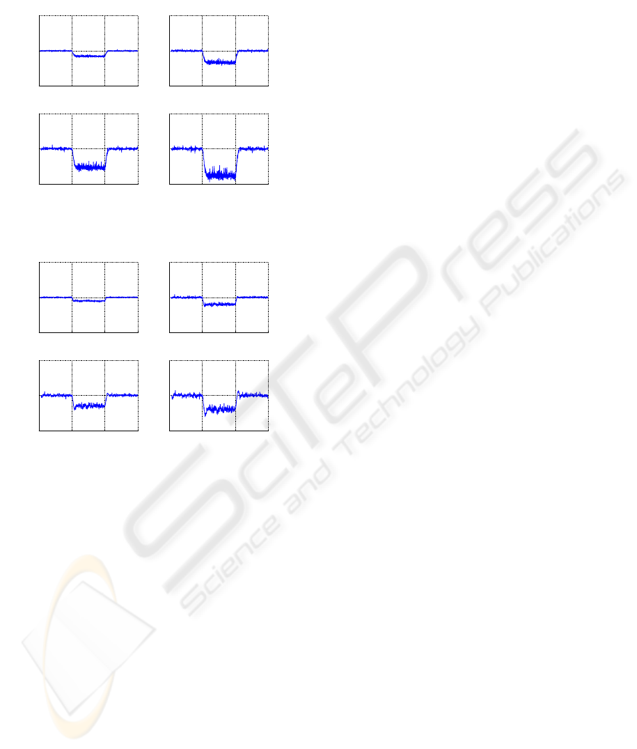
Figure 10: Synch. error with peer RCF and master RCF.

In Fig. 10 we simulate the algorithm where peer

RCF and master RCF are combined. We see a better

initialization compared with the result in Fig. 8 and

smaller error during the frequency drift compared to

Fig. 9. This confirms the improved performance we

expect for the combination of peer and master RCF

calculation.

7 CONCLUSIONS

In this paper, we have introduced two methods that

calculate the frequency ratio of two elements based

on the information contained in PTP messages. The

peer RCF calculation utilizes delay messages locally

and leads to fast convergence. The

master RCF

calculation use Sync messages to calculate the

frequency ratio between the grandmaster and the

slave. It performs better when there is constant

frequency drift in the master clock. It has been

shown both through analysis and simulation results

that a combination of both methods improves

synchronization performance. Future work could

illuminate the optimal combination of master RCF

and peer RCF estimation for widely different system

parameters or system requirements.

REFERENCES

Chen B., Chen Y.P., Xie J.M., Zhou Z.D., Sa J.M., 2005.

Control methodologies in networked motion control

systems. In: Proc. of 2005 International Conference

on Machine Learning and Cybernetics, Guangzhou.

IEEE, 1997. Standard for LAN/MAN CSMA/CD Access

Method, IEEE, New York.

IEEE, 2002. IEEE Standard for a Precision Clock

Synchronization Protocol for Networked Measurement

and Control Systems. IEEE, New York. ANSI/IEEE

Std 1588-2002.

IEEE, 2007. Standard for Local and Metropolitan Area

Networks - Timing and Synchronization for Time-

Sensitive Applications in Bridged Local Area

Networks, IEEE, New York.

IEEE, 2007. IEEE P1588

D2.2 Draft Standard for a

Precision Clock Synchronization Protocol for

Networked Measurement and Control Systems, IEEE,

New York.

Jasperneite J., Shehab K., Weber K., 2004. Enhancements

to the time synchronization standard IEEE-1588 for a

system of cascaded bridges. In: Proc. of 2004 IEEE

International Workshop on Factory Communication

Systems, Vienna.

Jasperneite J., Neumann P., 2004. How to guarantee real-

time behaviour using Ethernet. In: Proc. of 11th IFAC

Symposium on Information Control Problems in

Manufacturing (IN-COM2004), Salvador-Bahia.

Jasperneite J., Feld J., 2005. PROFINET: an integration

platform for heterogeneous industrial communication

systems. In: Proc. of ETFA 2005, 10th IEEE

International Conference on, Catania.

Mills, D.L., 1989. Internet time synchronization: The

network time protocol. Network Working Group

Request for Comments.

Mills, D.L., 1994. Precision synchronization of computer

network clocks. Available: citeseer.nj.nec.com/

mills94precision.html.

Na, C., Obradovic D., Scheiterer R.L., Steindl G. and

Goetz F.J., 2007. Synchronization Performance of the

Precision Time Protocol. In: 2007 IEEE International

Symposium on Precision Clock Synchronization for

Measurement, Control and Communication, Vienna.

Na, C., Obradovic D., Scheiterer R.L., Steindl G. and

Goetz F.J., 2008. Enhancement of the Precision Time

Protocol in Automation Networks with a Line

Topology. Submitted to: IFAC 2008, Seoul.

Nieminen, J., 2007. Synchronization of Next Generation

Wireless Communication Systems. Master thesis,

Helsinki University of Technology, Helsinki.

ICINCO 2008 - International Conference on Informatics in Control, Automation and Robotics