GPU-BASED NORMAL MAP GENERATION

Jesús Gumbau, Carlos González

Universitat Jaume I. Castellón, Spain

Miguel Chover

Universitat Jaume I. Castellón, Spain

Keywords: GPU, normal maps, graphics hardware.

Abstract: This work presents a method for the generation of normal maps from two polygonal models: a very detailed

one with a high polygonal density, and a coarser one which will be used for real-time rendering. This

method generates the normal map of the high resolution model which can be applied to the coarser model to

improve its shading. The normal maps are completely generated on the graphics hardware.

1 INTRODUCTION

A normal map is a two-dimensional image whose

contents are RGB colour elements which are

interpreted as 3D vectors containing the direction of

the normal of the surface in each point. This is

especially useful in real-time applications when this

image is used as a texture applied onto a 3D model,

because normals for each point of a model can be

specified without needing more geometry. This

feature enables the use of correct per-pixel lighting

using the Phong lighting equation.

Normal map generation is a key part in real-time

applications, such as video-games or virtual reality,

due to the intensive use of techniques such as

normal-mapping, used to increase the realism of the

scenes.

Compared to traditional per-vertex lighting, per-

pixel lighting with normal maps gives the rendered

model a great amount of surface detail, which can be

appreciated through the lighting interactions of the

light and the surface. Figure 1 shows the effect of

applying a normal, extracted from a highly detailed

model, onto a coarser mesh which is used for

rendering the model in real-time without almost

losing quality. This technique gives detail to meshes

without having to add real geometric detail.

Altough normal maps can be easily generated

when both the reference and the working meshes use

a common texture coordinate system, this is not

always the case and thus, it is not trivial to

implement on the graphics hardware. This is the

reason why this kind of tools are often implemented

on software.

The high programmability of current graphics

hardware allows for the implementation of these

kinds of methods on the GPU. This way, the great

scalability of the graphics hardware, which is

increased even more each year, can be used to

perform this task.

2 STATE OF THE ART

Some other authors have presented works about the

generation of normal maps for simplified meshes.

(Sander, 2001) (Soucy, 1996) (Cignoni, 1998)

generate an atlas for the model so that they can

sample the colour and normal values of the surface

to be stored in a texture, which will be applied over

a simplified version of the same original model.

However, these methods need the coarse version of

the mesh to be a simplified version of the sampled

mesh, which is a disadvantage. The method

proposed in this work does not have this limitation,

the only limitation; of our work is that the two

objects involved must have the same size, positions

and shape in the space.

Gumbau J., González C. and Chover M. (2008).

GPU-BASED NORMAL MAP GENERATION.

In Proceedings of the Third International Conference on Computer Graphics Theory and Applications, pages 62-67

DOI: 10.5220/0001097100620067

 SciTePress

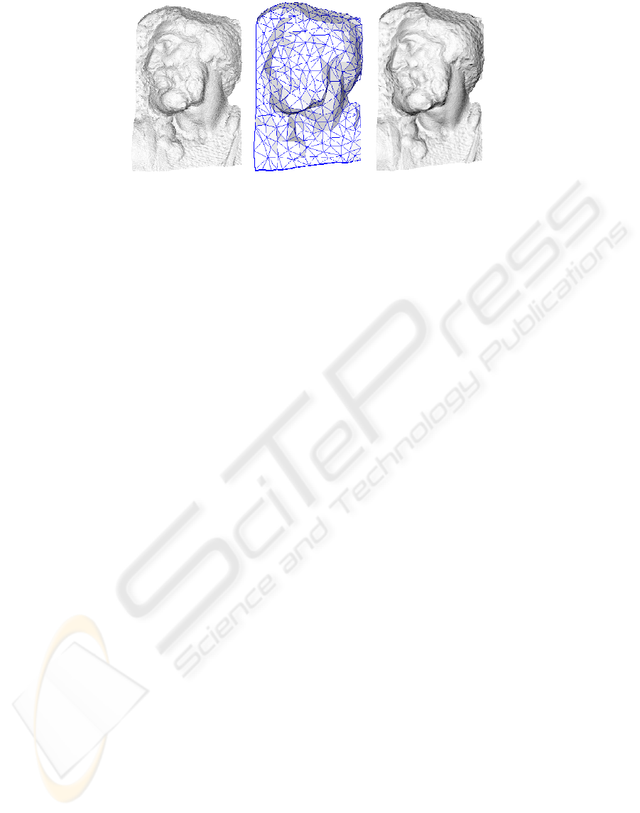
Figure 1: Normal mapping example: the figure on the right shows the results of applying the normal map generated from

the high resolution mesh (left) and its coarse representation (middle).

Although other authors (Wang, 2002)

implementation takes advantage of graphics

hardware for the generation of normal maps, they do

not exploit it completely as they only use the

rasterizing stage of the GPU, performing other tasks

on the CPU. Moreover, this method has some

limitations: it can not generate the normals for faces

that are occluded by other parts of the model, and it

does not fully take advantage of the graphics

hardware capabilities, having to perform some read

backs from the colour buffer.

On the other hand, (Gumbau, 2006) present an

extremely fast method to calculate normal maps on

the GPU. However, it has a strong limitation: the

normal map generated from a mesh A to be applied

to a mesh B can be generated if and only if the mesh

B has been generated from a simplification process

applied to the mesh A, and the distribution of texture

coordinates fulfil some special requirements. These

strong limitations enable the normal map to be

generated very fast, but it can only be used in very

specific and controlled situations.

Finally, there exist some applications (NVIDIA)

that use ray tracing to calculate the normal map in a

very precise way. Their disadvantage is that they do

not benefit from the graphics hardware, and thus

they will not be explained.

3 METHOD

The method presented in this paper generates the

normal map completely on the GPU, so that all the

work is performed by the graphics hardware. This

has the advantage of taking profit of a highly

parallelizable hardware which will quickly

increment its performance in the next years. Coarse

versions of highly detailed meshes are often

modelled from scratch (as in the video game

industry for example), so we can not expect any

correspondence between the two meshes other than

geometric proximity. Having this in mind, this

method avoids the requirement of generating the

coarse mesh from the highly detailed mesh, and, as a

consequence, they can be modelled separately.

3.1 Main Idea

Let M

and M

be two polygonal meshes so that

is a coarse representation of M

. We define

the normal map MN as a two-dimensional texture

which can be used as input for normal mapping. Our

goal is to calculate MN on the GPU.

We assume that M

is a good approximation of

and that both are situated in the same spatial

position, and have the same sizes and orientation.

Basically, to calculate MN, one render of M

will

be performed for each triangle (T) of M

discarding those parts of the model projected outside

T. For every fragment of M

projected through T,

the direction of the normal will be extracted and

stored into MN, using the texture coordinates of T to

calculate the exact position inside the texture. Easily

explained, the algorithm works as: the normals of all

those pixels of the high resolution mesh rendered

through the window formed by the triangle T will

become the part of the normal map applied to T.

This way, M

is used as a three-dimensional grid

which contains information about how to render

Texture coordinates of M

must be fully

unwrapped in a way that there are no triangles

overlapped in texture space.

3.2 Transformation Matrices

For each iteration of the algorithm, a transformation

matrix (which encapsulates the model, view and

projection transformations) must be calculated. This

matrix transforms the triangle T (composed by the

vertices v0, v1 and v2) to the two-dimensional

GPU-BASED NORMAL MAP GENERATION

triangle t (composed by the texture coordinates of T:

t0, t1 and t2).

Figure 2 shows this process. Once obtained, this

matrix will be applied to every vertex of M

, so

that all the triangles visible through T will be

projected onto the area defined by t.

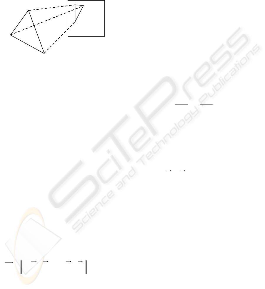
Figure 2: The transformation matrix which converts the

3D triangle T into a 3D triangle composed by the texture

coordinates of T must be calculated at each step.

3.2.1 Model/View Matrix Calculation

The model/view matrix (MV) is derived from the

three parameters that define a virtual camera which

will be configured so that its viewing direction is

parallel to the normal of T, looking to the center of

the triangle and located at a certain distance of T. As

we will use an orthographic projection, the distance

T will not affect the final projection.

To define a virtual camera, a third parameter is

needed: the roll angle usually specified as the “up

vector”. This vector is calculated using its texture

coordinates.

Let (t

, t

y t

) be the texture coordinates of the

three vertices of T (v

, v

). The vertical value on

our two-dimensional space will be assumed to be the

vector (0,1). Having this in mind we can propound

the following equation system:

⎪

⎭

⎪

⎬

⎫

−+−=

)·()·(1

)·()·(0

1312

yyyy

xxxx

tttt

βα

(1)

Working out the values of α and β will let to

calculate the desired vector in the following way:

)·()·(

1312

vvvvUP −+−=

βα

(2)

3.2.2 Projection Matrix

We will use a pseudo-orthogonal projection matrix

to project the vertices of M

. Similar to an

orthogonal matrix, it will not modify the X and Y

coordinates depending on the value of Z. However

its behavior is not exactly the same of a common

orthogonal matrix, as we will explain later.

We need to calculate a projection matrix (P)

which transforms the coordinates of T into its

texture coordinates t, so we propound the following

equations:

}2,1,0{· ∈∀= itvP

(3)

The problem here is that the matrix P is a

homogeneous transform matrix (it has 16 elements),

and thus it can not be solved directly because we

have not enough equations.

As we are looking for a pseudo-orthogonal matrix

which transforms the X and Y coordinates of each

vertex to the texture coordinates, we only need to

calculate the value of the 6 unknowns (P

) shown in

figure 3:

⎟

⎠

⎞

⎜

⎝

⎛

⎟

⎠

⎞

⎜

⎝

⎛

⎟

⎠

⎞

⎜

⎝

⎛

−

1000

FED

CBA

PPP

Figure 3: Unknowns to solve to calculate the desired

projection matrix.

where i refers to each one of the three vertices of

T, and w

refers to those vertices pre-multiplied by

the MV matrix, as shown below:

}3,2,1{· ∈∀= iwvMV

(4)

and Nt

are the normalized device

coordinates for each one of the transformed vertices.

As after perspective division, the visible coordinates

in the screen are situated in the range [-1,1].

Nevertheless, we want them to be in the range [0,1]

of the texture coordinates, then we have to take that

into account. They are calculated using the

following formula:

}3,2,1{1),·(2),( ∈∀−= ittNtNt

(5)

After solving the equations propounded in

Figure 3 we get the desired pseudo-orthogonal

matrix which projects every vertex of M

in a way

that all the triangles visible through T will be

rendered inside the area formed by the texture

coordinates of T.

Texture s

ace

GRAPP 2008 - International Conference on Computer Graphics Theory and Applications

3.3 Framebuffer

As explained before, the number of renders of M

needed to be performed is equal to the triangle count

of M

. However, we are only interested in the

pixels which are inside the area formed by the

triangle T projected with the matrix MVP. Setting up

the stencil buffer to discard all pixels which are

outside the projection of T, is a very simple way to

discard unwanted pixels and to protect those parts

which have been already rendered.

Finally, the pixel shader re-scales every un-

masked normal to the range [0,1], so that the normal

vector can be encoded as a colour in the RGB space.

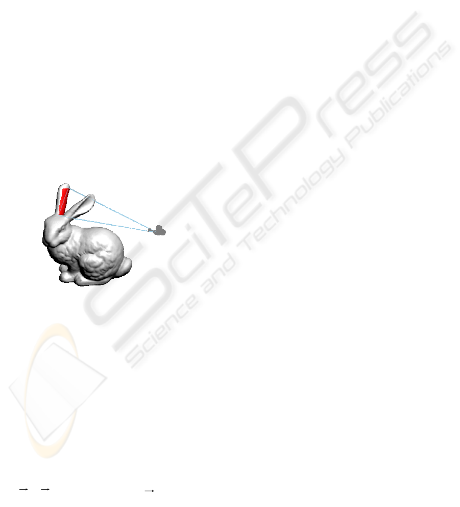
3.4 The Auto-occlusion Problem

Sometimes, there are some parts of the models that

will cause this method to fail. This happens when

there is another part of the model between the

camera and the real target surface. This problem is

clearly shown in Figure 4, where a part of the model

is incorrectly occluding the desired surface

(coloured in red), causing the normal map to be

completely invalid.

Figure 4: Auto-occlusion problem: the ear next to the

camera is occluding the real desired geometry.

To solve this problem we have developed a

technique called vertex mirroring. Basically we

consider that if a pixel is going to be drawn more

than once (some parts of the model overlap in screen

space), then the valid pixel will be that one which is

closer to T. This is similar to what raytracing-based

normal map generation algorithms do: if some

polygons intersect the ray, take the one which is

closer to T.

Let Π be the plane containing T. Let N be the

normal of Π, v

be each one of the vertices of M

and k

be the distance between Π and v

. Then the

final position of v

is recalculated as follows:

Nkkclampvv

iiii

)·,0,(·2−=

(6)

The function clamp(a,b,c) will trunk the value a

inside the range [b,c]. This ensures that all vertices

of M

are in front of the plane Π, because those

vertex that are behind that plane are mirrored

through it. After performing this step, we can use the

standard depth test to ensure that each rendered pixel

is the nearest possible to T.

This technique can be implemented in a vertex

shader for optimal performance, in a clear, elegant

and efficient way.

3.5 Normal Map Border Expansion

Once the previous process is over, the normal map is

correctly calculated. However, due to the texture

filtering methods used in real-time hardware,

normals could incorrectly interpolate with their

neighbouring “empty” texels. To solve this problem,

we need to create an artificial region surrounding

every part of the normal map.

To detect those texels that do not contain a valid

normal, an extra pass rendering a full screen quad

textured with the previously generated normal map

will be performed. For each pixel, the pixel shader

of the normal map generator will check if the texel

belonging to the pixel being processed has a module

less than 1, which means that it does not contain a

valid normal (because all normal must be unitary). If

that happens, the pixel must be filled with the

average normalized value of its neighbouring texels

which contain a valid normal.

At the end of the process a 1-pixel sized frontier

is created around all parts of the normal map that

didn’t contain a valid normal. This process can be

repeated with the resulting texture to expand the

frontier to a user defined size.

4 RESULTS

All tests were performed on an Athlon64 3500+ /

1GB RAM / GeForce 6800 Ultra and can be divided

into two categories: performance and quality tests.

Table 1 shows a study of total times required to

generate the normal maps for two models with a

different polygonal complexity. For each model

, first column) different coarse approximations

are used (M

, second column) to generate MN. The

column on the right shows the time in milliseconds

needed to calculate the normal map for a certain

combination of meshes.

An octree-based acceleration structure is used to

discard as many triangles as possible in an efficient

way to improve rendering times up to 10 times.

GPU-BASED NORMAL MAP GENERATION

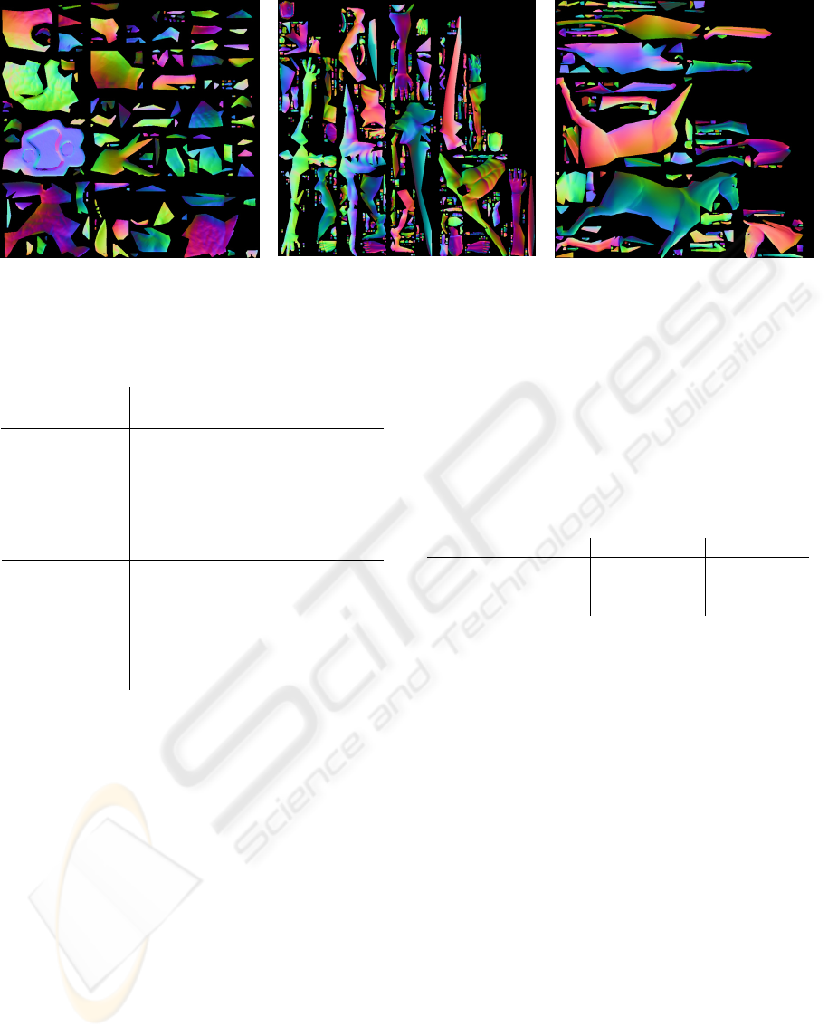
Figure 5: Normal maps used in Figure 6. From left to right: the bunny, the monster and the horse.

Table 1: Total times in milliseconds needed to generate

the normal maps for two different models, using a set of

different coarse approximations.

Triangles

Triangules

Time

(ms)

250 140

500 224

1.000 442

2.000 721

2.500 912

69.451

3.000 1034

250 22

500 32

1.000 66

2.000 102

2.500 131

16.843

3.000 158

On the other hand, some tests have been done to

compare our results with a software based approach,

which is implemented in the nVidia Melody tool.

These results are not shown in a table because that

tool does not display time information. However,

those the times needed for the application to

calculate the normal maps for the same high

resolution model used in our tests vary from 2 to 6

seconds for the worst and better cases, which is

worse compared with our results.

The other studied parameter is how the size of

the normal map affects to our method. As one can

imagine, the bottleneck of our application is the

huge amount of vertices needed to be processed,

because the pixel operations performed are very

light weight. Table 2 shows how our method is

independent of the size of the normal map.

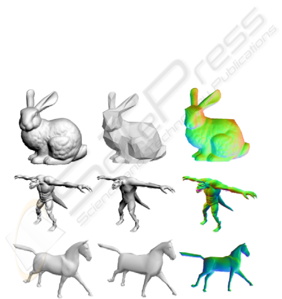
Figure 6 shows the results of the generated

normal maps for 3 different models: the bunny, the

monster and the horse. The column on the left shows

the high resolution models (M

). The column on

the centre shows the coarse versions of each mesh

) used to calculate the normal map. Finally, the

column on the right shows the final normal map

applied to the coarse mesh, so one can check the

final visual quality of the normal map. Figure 5

shows the normal maps generated for its use in

Figure 6.

Table 2: Generation times at different resolutions.

Triangles M

/ M

Resolution Time (ms)

128 x 128 442

512 x 512 441

69.451 / 1.000

1024 x 1024 443

5 CONCLUSIONS

We have presented a GPU-based method for normal

map generation. This method exploits the graphics

hardware in a way that it takes advantage of the

parallelization of the GPU in various ways. On the

one hand, the graphics hardware utilizes several

shading processors in parallel, which is inherent to

the graphics pipeline. On the other hand, there is a

parallelization between the GPU and the CPU,

which is useful to calculate matrices on the CPU

while the GPU is performing each render. Moreover,

the method proposed here does not have some of the

limitations explained in the introduction.

Although this method has been used to calculate

the normals of a high resolution polygonal mesh, it

could also be used to obtain other surface parameters

such as diffuse colour maps, height maps or specular

maps. As seen before, this method is highly

dependent of the number of triangles of both models

and M

). However, this limitation can be

GRAPP 2008 - International Conference on Computer Graphics Theory and Applications

reduced by using some kind of hierarchical culling

method to discard most of the unneeded geometry.

In this article we have used octrees as an

acceleration structure. Moreover, reducing the

number of renders needed by grouping triangles of

would also be possible. This would highly

accelerate the total generation times, although this

has been left as future work.

ACKNOWLEDGEMENTS

This work has been supported by the Spanish

Ministry of Education and Science (MATER project

TIN2004-07451-C03-03, TIN2005-08863-C03-03),

the European Union (GAMETOOLS project IST-2-

004363), the Jaume I University (PREDOC/2005/12,

PREDOC/2006/54) and FEDER funds.

REFERENCES

Sander, P.V., Zinder, J., Gortler, S.J., Hoppe, H., 2001.

Texture mapping progressive meshes. SIGGRAPH

2001.

Soucy, M., Godin, G., Rioux, M., 1996. A texture-

mapping approach for the compression of colored 3D

triangulations. Visual Computer, 12.

Cignoni, P., Montani, C., Scopigno, R., 1998. A general

method for preserving attribute values on simplified

meshes. Visualizaton’98 proceedings, IEEE.

Wang, Y., Fröhlich, B., Göbel, M., 2002, Fast Normal

Map Generation for simplified meshes. Journal of

Graphics Tools.

Gumbau, J., González, C., Chover, M., Fast GPU-based

normal map generation for simplified models,

WSCG’2006 Posters proceedings.

Cohen, J., Olano, M., Manocha, D. Appearance Preserving

Simplification, SIGGRAPH 98.

Becker, G., Nelson, M. Smooth Transitions between

Bump Rendering Algorithms, SIGGRAPH 93.

NVIDIA, NVIDIA Melody, http://developer.nvidia.com.

Figure 6: The column on the left show the high resolution models (M

). The column in the middle shows the coarse

versions (M

) of those meshes. Finally, the column on the right show the resulting normal map applied to M

GPU-BASED NORMAL MAP GENERATION