DETERMINE TASK DEMAND FROM BRAIN ACTIVITY

Matthias Honal and Tanja Schultz

Carnegie Mellon University, 407 South Craig Street, Pittsburgh 15213, PA, USA

Karlsruhe University, Am Fasanengarten 5, 78131 Karlsruhe,Germany

Keywords: Human-centered systems, Brain Activity, EEG, Task Demand Identification, Meeting and Lecture Scenario.

Abstract: Our society demands ubiquitous m

obile devices that offer seamless interaction with everybody, everything,

everywhere, at any given time. However, the effectiveness of these devices is limited due to their lack of

situational awareness and sense for the users’ needs. To overcome this problem we develop intelligent

transparent human-centered systems that sense, analyze, and interpret the user’s needs. We implemented

learning approaches that derive the current task demand from the user’s brain activity by measuring the

electroencephalogram. Using Support Vector Machines we can discriminate high versus low task demand

with an accuracy of 92.2% in session dependent experiments, 87.1% in session independent experiments,

and 80.0% in subject independent experiments. To make brain activity measurements less cumbersome, we

built a comfortable headband with which we achieve 69% classification accuracy on the same task.

1 INTRODUCTION

Our modern information society increasingly

demands ubiquitous mobile computing systems that

offer its users seamless interaction with everybody,

everything, everywhere, at any time. Although the

number and accessibility of mobile devices such as

laptop computers, cell phones, and personal digital

assistants grows rapidly, the effectiveness in

supporting the users to fulfilling their tasks proves to

be much smaller than expected. This mainly results

from the fact that such devices lack situational

awareness and sense for the users’ needs. As a

consequence users waste their time with manually

configuring inflexible devices rather than obtaining

relevant information and efficient automatic support

to solve their problems and tasks at hand.

It is our believe that the solution lies in intelligent

trans

parent human-centered systems that sense,

analyze, and interpret the needs of their users, then

adapt themselves accordingly, provide the optimal

support to given problems, and finally present the

relevant results in an appropriate way. The goal of

the work presented here is to solve the analytical

part of human-centered systems, i.e. sensing,

analyzing, and interpreting the users’ needs.

For this purpose we develop learning approaches

hat derive the users’ condition from their brain

activity. We are interested in conditions that are

important in the context of human-computer

interaction and human-human communication. In

this particular study we focus on the (mental) task

demand as a user condition in the context of lecture

presentations and meetings.

The term task demand defines the amount of mental

resources require

d to execute a current activity.

Although we are using the general term task de-

mand, we are exclusively concerned about the men-

tal not the physical task demand. Task demand infor-

mation can be helpful in various situations, e.g.

while driving a car, operating machines, or perform-

ing other critical tasks. Depending on the level of

demand and cognitive load, any distraction arising

from electronic devices such as text messages, in-

coming phone calls, traffic or navigation informa-

tion, etc. should be suppressed or delayed. Also, the

analysis of task demand during computer interaction

allows to asses usability. In a lecture scenario, a

speaker may use task demand information to tailor

the presentation toward the audience.

In this paper we investigate the potential of detecting

ask demand by measuring the brain activity using

scalp electrodes. Although we focus on the system

evaluation in the lecture and meeting scenario, the

described methods are applicable to any other real-

life situation. To make electrode-based recordings

acceptable, the following issues must be addressed:

100

Honal M. and Schultz T. (2008).

DETERMINE TASK DEMAND FROM BRAIN ACTIVITY.

In Proceedings of the First International Conference on Bio-inspired Systems and Signal Processing, pages 100-107

DOI: 10.5220/0001069001000107

 SciTePress

• Robustness: The system needs to be robust against

artefacts introduced by speech or body movement

• Usability: EEG sensors and recording device need

to be user friendly and comfortable to wear

• Applicability: Measuring brain activity must be

feasible in realistic scenarios in real-time.

In this work we are addressing these three goals by

relaxing the inconveniences of clinical brain activity

recording and make it applicable to real human-

computer interaction and human-human communi-

cation scenarios.

2 ELECTROENCEPHALOGRAM

The source of the Electroencephalogram (EEG) is

neural activity in the cortex, the outmost part of the

human brain. This neural activity causes electrical

potential differences, which can be measured using

scalp electrodes. Information between neurons is

transferred via the synapses where chemical

reactions take place causing ion movements. These

movements result in excitatory or inhibitory

electrical potentials in the post-synaptic neurons.

The electrical fields emerging from the ion

movements are called cortical field potentials and

have a dipole structure. If the electrical activity of a

huge number of neurons is synchronized, the

corresponding dipoles point all in the same

direction. Their sum becomes large enough such that

potential differences between particular scalp

positions and a constant reference point can be

measured. EEG characteristics like frequency,

amplitude, temporal and topographic relations of

certain patterns can then be used to make inferences

about underlying neural activities (Zschocke, 1995).

In the EEG which can be measured at the scalp,

amplitudes between 1μV and 100μV and fre-

quencies between 0Hz and 80Hz can be observed.

These EEG signals show specific characteristics at

different scalp positions, depending on the current

mental condition. When the human brain is not

absorbed by external sensory stimuli or other mental

processes, we usually observe the α-activity across

the cortex, i.e. rhythmic signals between 8Hz and

13Hz with large amplitudes. When performing

higher mental processes the α-activity is attenuated

and other activity patterns occur in those cortex

regions, where the processes happen. In many cases

these patterns are identified by γ-activity, which

typically show frequencies around 40Hz and have a

lower amplitude than α-activity (Schmidt and

Thews, 1997). In this work we assume that the de-

gree of α-activity attenuation and activity at higher

frequencies is correlated with task demand. This is

justified by the fact that the amplitude of non-α-

activity is correlated with the degree of vigilance, a

physiological continuum between sleepiness and

active alertness (Zschocke, 1995). Furthermore, it is

known that people are more alert when the task

demand is high. The frequency analysis of our

recorded data confirms this assumption. During most

activity types several cortex regions are involved

and task demand is characterized by the amplitude

of non-α-activity in all regions involved in the

current task. This suggests that the activity of the

whole cortex must be taken into account to achieve

optimal results for task demand estimation.

3 TASK DEMAND & VIGILANCE

A large body of research work concerns the

computational analysis of brain activity, applying

EEG, functional magnetic resonance imaging, and

functional near infrared spectroscopy to areas such

as estimation of mental task demand. Several groups

reported research on the computational assessment

of task demand based on EEG data recorded while

varying the task difficulty (Smith, 2001), (Pleydell-

Pearce, 2003), (Berka, 2004). These studies focused

on the design of intelligent user interfaces that

optimize operator performance by adjusting to the

predicted task demand level. Regression models

were trained to predict task demand from the

recorded EEG data. These models used the task

difficulty or the rate of errors as references during

task execution. The features extracted from the EEG

data represented mostly the frequency content of the

signals. Positive correlations between predictions

and references or predictions and self-estimates of

task demand (Smith, 2001) are reported throughout

these studies. Pleydell-Pearce (2003) achieved a

classification accuracy of 72% for the discrimination

of low versus high task demand in subject and

session dependent experiments and 71% in subject

independent experiments. Task demand assessment

has also been done on data from other modalities,

including muscular activity (Pleydell-Pearce, 2003),

blood hemodynamics (Izzetoglu, 2004), and pupil

diameter (Iqbal, 2004). Reasonable results could be

achieved with all three modalities. However,

correlations between pupil diameter and task

demand could only be shown for one interactive task

out of a group of various cognitive tasks.

Other work focused on the EEG-based estima-

tion of operator’s vigilance during sustained atten-

tion tasks (e.g. car driving or operating a power

plant). Jung (1997) asked subjects to respond to

auditory stimuli which simulate sonar target

detection, while EEG was recorded from five

DETERMINE TASK DEMAND FROM BRAIN ACTIVITY

101

electrodes over the parietal, central and occipital

cortex. The error rate in terms of failures to respond

to stimuli was then used as reference for a Multi-

Layer ANN which was trained with a frequency

representation of the EEG signals to predict a

vigilance index between 0 and 1. On unknown data a

root mean square error (RMS-error) of 0.156

between predictions and references is reported for a

subject dependent experimental setup. Duta et al.

(Duta, 2004) recorded EEG from the mastoids while

subjects had to perform visual attention tasks.

Vigilance was labelled by experts who visually

inspected the recorded data. Three vigilance

categories “alertness”, “intermediate” and “drowsi-

ness” were distinguished. Using the coefficients of

an AR model as features for Multi-Layer ANNs

39% to 62% predictions matched the references in

subject independent experiments.

4 DATA & METHODS

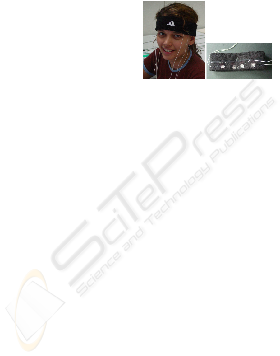
4.1 Data Capturing

Two different devices were used for data

acquisition: an EEG-cap from ElectroCap™ and a

self-made EEG-headband (see Figure 1). The majo-

rity of data were recorded with the ElectroCap™

using 16 electrodes placed at positions fp1, fp2, f3,

f4, f7, f8, fz, t3, t4, t5, t6, p3, p4, pz, o1, and o2 ac-

cording to the international 10-20 system (Jasper,

1958). Reference electrodes were attached to the ear

lobes and linked together before amplification.

Although we are aware of the relationship between

facial expressions and level of task demand, we

decided to exclude the motor cortex from our mea-

surement for two reasons: firstly, the facial muscular

activity is partly captured by the frontal EEG

electrodes, and secondly we assume that motor

activity is of rather minor importance for the

assessment of our classification task.

Some data were recorded with a headband, in

which we sewed in four electrodes at the forehead

positions fp1, fp2, f7, and f8. Reference electrodes

were attached to the mastoids and linked together

before amplification, the ground electrode was

placed at the back of the neck. The headband has

three major advantages over the ElectroCap™ which

are crucial to real-life applications: the headband is

(1) more comfortable to wear, (2) much easier to

attach, and (3) better to maintain and clean, also no

electrode gel gets in contact with the subject’s hair.

The drawback is the limited positioning and number

of electrodes compared to the ElectroCap™.

Figure 1: Headband, build-in electrodes at fp1, fp2, f7, f8.

In contrast to recordings for clinical purposes,

subjects were allowed to move freely during the

recordings to keep the situation as natural as

possible, i.e. the subject's head was not fixated.

Consequently we had to deal with data artefacts

introduced by muscular activity (some recordings

required speaking as well). Strategies to remove

those artefacts will be described in section 4.2.

Amplification and A/D-conversion was done

with a 16 channel VarioPort™ physiological data

recorder (Becker, 2005). Each channel had an

amplification factor of 2775 and a frequency range

from 0.9Hz to 60Hz. After amplification, A/D

conversion was performed using 4096 A/D-steps

and a sampling rate of 256 Hz. The data was

transferred instantaneously from the amplifier to a

computer via an RS232 port for online processing.

The port capacity is limited to 115200 Bits per

second which corresponds to 28 electrode channels

at a sampling of 256Hz. Although sampling with a

lower frequency should be sufficient to avoid

aliasing when considering the amplifier’s upper

cutoff-frequency of 60Hz, we decided to go with

256Hz since for technical reasons the slope of the

band pass filter is very small.

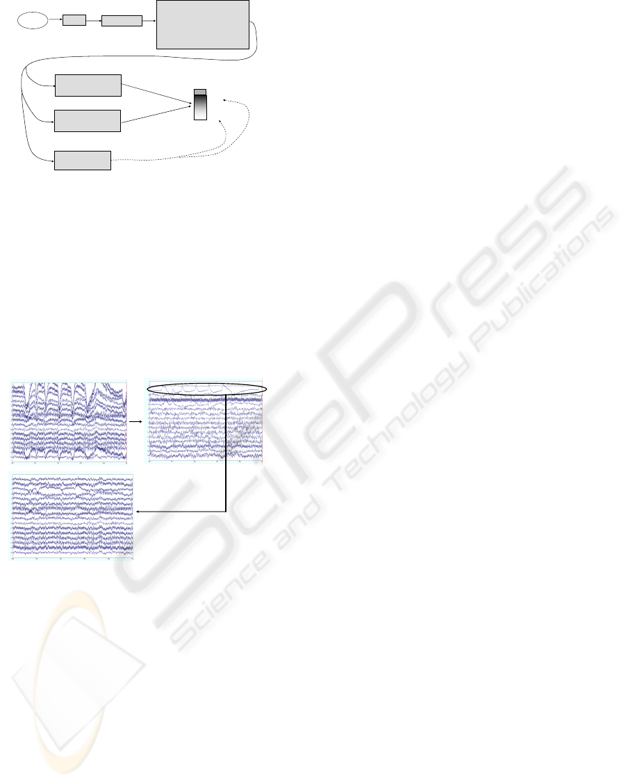
4.2 Data Preprocessing

Figure 2 summarizes the signal processing steps of

our task demand estimation system. After EEG

recording, artefacts are removed applying inde-

pendent component analysis (ICA). A short time

Fourier transform (STFT) is used for feature

extraction. After feature normalization and

averaging over temporally adjacent features,

different methods for reducing the dimensionality

are used. Finally, Support Vector Machines (SVMs)

or Artificial Neural Networks (ANNs) for

classification or regression are applied to obtain task

demand predictions. We also applied Self-

Organizing-Maps (SOMs) to determine which levels

of task demand can be reliably discriminated.

BIOSIGNALS 2008 - International Conference on Bio-inspired Systems and Signal Processing

102

EEG

Artifact Removal

ICA

averaging

normalization

dimensionality reduction:

• av. over freq. bands

• lin discr. analysis

• correlation based

ANNs

SVMs

Classification

Task Demand

low

medium

high

Overload

Task Demand

low

medium

high

Overload

Regression

ANNs

SVMs

STFT

Feature Extraction

Self-Organizing

Maps

Data Analysis

determine task demand levels to be distinguished

Figure 2: Task Demand Estimation System.

4.2.1 Artefact Removal

Artefacts such as muscular activity and especially

eye movements contaminate the EEG signal, since

the corresponding electrical potentials are an order

of magnitude larger than the EEG sources. This

causes in particular problems in the EEG that is

measured over the frontal cortex. ICA has shown to

be very efficient for artefact removal in EEG data

(Jung et al., 2000).

Original data ICA components

Back projected data

Removal of component 2

Figure 3: Artefact removal applying ICA: (1) independent

components are computed from the original data (top left),

(2) the second component (eye blinking artefact) is identi-

fied and rejected (top right), and (3) the data is projected

back to the original space (bottom left).

To apply ICA to EEG data it is assumed that the

signal measured at one electrode can be described by

a linear combination of signals emerging from

independent processes (i.e. cortical field potentials,

muscular artefacts, 60Hz AC noise): Let x(t) be the

vector of signals measured at all electrodes at time t

and s(t) be the independent components. Then x(t)

can be expressed by x(t) = A · s(t), where A is called

mixing matrix. ICA computes the matrix A, or its

inverse the de-mixing matrix W, such that

independent components can be estimated from the

measured signals (Hyväarinen et al., 2000). Artefact

components can then be identified either by visual

inspection of the training data or by using cross-

validation and be rejected from the data. The re-

maining components are projected back into the

original coordinate system (see Figure 3). For ICA

computation we used the open source Matlab tool-

box EEGLAB (Delorme et al., 2004), which applies

the Informax algorithm to the matrix estimation.

4.2.2 Feature Extraction, Averaging and

Normalization

After artefact removal we computed the power

spectrum of the time signal applying STFT. For two-

second long segments overlapping by one second,

features were computed representing the content of

frequency bands with 0.5Hz width. This results in

one feature vector per second. The dimensionality of

one feature vector for 16 electrode channels and

frequencies ranging from 0 to 45Hz is 16·90=1440.

To reduce the influence of outliers final feature

vectors for each time point were obtained by

averaging over k previous features. To compensate

for different ranges in the frequency bands, we

normalized each feature using the following two

normalization approaches:

• GlobalNorm: Feature means and variances are

calculated based on the complete training set.

Calculated values are used globally for mean

subtraction and variance normalization on all data

(training, validation, and test data).

• UserNorm: Feature means and variances are

calculated on training, validation, and test data

separately for each user. Then, user-specific mean

subtraction and variance normalization is applied.

4.2.3 Feature Reduction

Since the dimensionality of the feature vector may

be large compared to the amount of training data, we

investigated various feature reduction methods. A

straightforward approach is to average over adjacent

frequency bands, another approach is the Linear

Discriminant Analysis (LDA), which selects features

according to their discriminative power (Fukunaga,

1972). For sparse data and large dimensionalities,

LDA estimation may become ill-conditioned.

Therefore, we also applied a correlation-based

feature reduction method, which selects those

features that correlate best with the variable to be

predicted. This method proved to be particular use-

ful for the assessment of task demand, since – in

contrast to LDA – it takes into account the

continuous nature of the predicted variable.

DETERMINE TASK DEMAND FROM BRAIN ACTIVITY

103

4.3 Data Analysis

To learn more about the data structure and to gain

insights into the granularity and distinctness of task

demand levels, we generated self-organizing maps

(SOMs) (Kohonen, 1995) for the training data. After

obtaining the Best Matching Unit (BMU) for each

training example, a map was calculated which

visualizes colour-coded clusters corresponding to

different task demand levels. Thus the spatial

relation between the feature vectors belonging to the

different task demand levels can be visualized

concisely on a two dimensional grid. Although the

SOM-based analysis may indicate which task

demand levels are easy to discriminate, the

hypotheses have to be verified experimentally on

test data. SOM training and visualization were

performed with the MATLAB™ based SOM-

Toolbox (Vesanto et al., 2000).

4.4 Learning Methods

We investigated two types of classifiers: Multilayer

ANNs and SVMs. ANN classifiers were trained with

standard back-propagation, based on feed-forward

networks with a

tanh activation function and one

hidden layer. For all ANNs early stopping

regularization was performed and the number of

neurons in the hidden layer was determined on the

validation data. For SVM-based classification we

used an implementation of SVM

light

(Joachims,

1999), which directly addresses the multi-class

problem (Tsochantaridis, 2004). SVMs were

restricted to linear kernels to limit computational

costs and avoid extensive parameter tuning. By

treating the task demand levels as class labels (e.g.

“low”, “medium”, “high”), both classification

methods can be applied to the problem of task

demand estimation. To exploit the information

contained in the ordinal scaling of the different class

labels, we investigated the regression versions of

ANNs and SVMs as well.

Since ANN predictions fluctuate due to random

weight initializations, predictions from five

networks trained on the same data were combined

using majority decisions (in case of classification) or

averaging (in case of regression).

4.5 Evaluation Methods

The system performance for task demand

assessment is evaluated in terms of classification

accuracy. When regression methods are used, class

labels are assigned numeric values and each

prediction is assigned to the label with the closest

value. Although confusion matrices could lead to a

deeper understanding of pros and cons of the

prediction methods, we decided to use the more

concise classification accuracies. Results presented

here are averages over all test sets and all class

accuracies. The latter gives more reliable results in

the presence of unbalanced test sets.

We use the normalized expected loss to compare

accuracies that were calculated based on different

numbers of classes. Comparing accuracies directly

would not be appropriate since the chance accuracy

(c)

varies with the number of classes. The

normalized expected loss relates the observed error

to the chance error and thus makes it independent

from the number of classes. The value of the

normalized expected loss is bound by 1/ A

(c)

and

ranges between 0 and 1.

5 EXPERIMENTS

We conducted various experiments to evaluate task

demand assessment and collected EEG data for this

purpose, using both the headband and the

ElectroCap™. In offline experiments we analyzed

and optimized the processing steps of the system.

5.1 Data Collection

Task demand data was collected from subjects

perceiving an audio-visual slide presentation. The

presentations were tailored to the subjects’

educational background and designed to provoke

each task demand level with equal amount of time.

The presentations were video-taped so that each of

the subjects could evaluate their task demand

afterwards by watching the tape. We defined the

following task demand levels:

• Low: All details of the presentation are well

understood with low mental effort.

• Medium: Some mental effort is required to

follow the presentation, not all details may be

understood.

• High: All available mental resources are required

to understand at least the essence of the topic.

Most of the details are not understood.

• Overload: The presentation topic is not

understood. The subject is overwhelmed,

disengaged and makes no more effort to

understand the presentation.

In total 7690 seconds of data were recorded with the

ElectroCap™ from six students (three male, three

female) between 23 and 26 years old. One subject

was recorded twice. 1918 seconds of data were

recorded with the headband from two students (one

male, one female) between 21 and 28 years old.

BIOSIGNALS 2008 - International Conference on Bio-inspired Systems and Signal Processing

104

5.2 Experimental Setup

One major goal of our experiments was to

investigate the impact of user and session

dependencies on the system performance. The other

goal was to examine the efficiency and performance

of the headband compared to the ElectroCap™. We

therefore conducted user/session dependent and

independent experiments on ElectroCap™ and

headband recordings using the following setup:

UD: User and session dependent setup: Different

subsets of the same session were used for training

(80%), validation (10%), and testing (10%). Four

sessions were recorded with the ElectroCap™ and

two with the headband.

UI: User and session independent setup: The system

was trained on three of the four ElectroCap™

recording sessions and tested on the fourth session

in a round-robin fashion. For better comparability

the same test sets as for setup UD were used.

Validation was performed on two held-out

ElectroCap™ recording sessions.

SI: Session independent but user dependent setup:

One subject was recorded twice in two separate

sessions using the ElectroCap™. The system was

trained on one session and tested on the other,

without validation set.

5.3 Results – Data Analysis

Figure 4 compares for one subject the SOM trained

on all task demand levels (left-hand side) to the

SOM trained on high and low task demand level

(right-hand side). The grey-scaled dots represent the

best matching units (BMUs) on the grid belonging to

the feature vectors of different task demand levels.

The size of the dots is proportional to the amount of

feature vectors that share the same BMU. Obviously

we see a large overlap between the BMUs when all

four task demand levels are considered, while the

BMUs for low and high task demand seem to be

well separable. Same observations were made for

the SOMs trained on other subjects.

Baseline results on the UD setup (no averaging,

GlobalNorm normalization, no feature reduction,

linear classification SVMs) confirmed our

expectation that the four task demand levels are

difficult to discriminate (classification accuracy

40%, normalized expected loss 0.81). When

distinguishing low versus high task demand we

achieved a classification accuracy of 78% and a

normalized expected loss of 0.43. The major reason

for the poor results on discriminating all four levels

is that subjects had difficulties to identify the

boundaries between adjacent demand levels. To

investigate this we asked some subjects to re-

evaluate their task demand at a later time. We found

a low intracoder agreement among adjacent task

demand levels, while high versus low task demands

were rarely confused. In the remainder of this

section we will therefore focus on the discrimination

between low and high task demand.

Figure 4: SOM trained on all four task demand levels (left-

hand side) and on low vs. high task demand (right-hand

side). Grey scale intensity indicates task demand level,

ranging from low (light) to overload (dark).

Table 1 shows the average amount of data per

subject after removing the medium and overload

task demand recordings.

Table 1: Data per subject (in seconds) for all setups.

Setup Training Validation Test

UD 247 31 64

UI 740 229 64

SI 257 - 48

5.4 Results – Learning Method

Table 2 compares the regression and classification

versions of ANNs and SVMs for the baseline system

(no averaging, GlobalNorm normalization, no

feature reduction). For all three experimental setups

SVMs perform better than ANNs. For setup SI the

regression SVMs significantly outperform the

classification SVMs. For the other setups the

differences between the two SVM variants are rather

small. Since at least theoretically the regression

SVMs should be able to better exploit the ordinal

scaled information given in the task demand levels,

we decided to use these in the remainder of our

experiments.

DETERMINE TASK DEMAND FROM BRAIN ACTIVITY

105

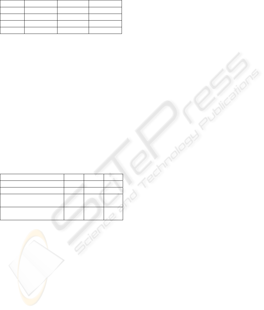
Table 2: Baseline system performance for all setups;

classification (

) and regression methods (

); In

parentheses: standard deviation for five ANN experiments.

Setup UD UI SI

SVM c 81% 72% 66%

SVM r 79% 74% 73%

ANN c 78% (7%) 70% (3%) 53% (5%)

ANN r 71% (3%) 69% (3%) 66% (5%)

5.5 Results – Normalization and

Feature Reduction

In the following experiments we optimized the

processing steps of our system in a greedy fashion

on the validation set. Table 3 shows the

classification accuracies for all experimental setups

with the optimal parameters (given in parentheses).

Averaging over k=2 feature vectors improved the

results for the UD and UI setup. The use of

normalization method UserNorm instead of the

baseline method GlobalNorm improved results for

setups UI and SI. This matches our expectation,

since this method reduces the variability across

sessions (UI and SI) as well as across subjects (UI).

Normalization is not relevant for the user dependent

setup (UD) since it only applies when data of

different subjects are used for training and test.

Table 3: Results for the optimized task demand system.

Setup UD UI SI

Baseline 78% 74% 73%

Averaging (k=2) 82% 79% 73%

Normalizing

(UserNorm)

N/A 80% 87%

Feature Reduction

(Corr-based)

92% 77% 66%

Feature reduction was only successful for UD,

where a correlation based reduction from 1440 to 80

features yielded considerable improvements. For the

other setups feature reduction did not help, probably

since despite normalization the data variability was

too large. Consequently, features which were well

correlated with task demand on the training data

exhibited poor correlations with task demand on the

test data. Comparing the results of feature reduction

among the different setups is difficult since the

optimal number of 80 features for the UD setup was

determined on the validation set, while we set this

number manually to 240 for the SI and UI setup as

the validation method did not give any reasonable

optimum.

Averaging over adjacent frequency bands for

feature reduction corresponds to putting features into

bins of size b. We observed that even for large

numbers of b the results did not drop much for any

of the setups. For b=45 (two features per electrode,

i.e. lower and the upper frequencies) results are in

the same range as without feature reduction. For

b=90 (one feature per electrode, 8 features in total)

results dropped significantly. This suggests that it is

sufficient to consider for task demand estimation the

content of two broad frequency bands: the lower

frequencies (around the α-band) and the higher

frequencies (around the γ-band). Experiments to

investigate this hypothesis are planned. The feature

reduction would benefit from more reliable model

estimation and reduced computational costs.

5.6 ElectroCap™ versus Headband

After optimizing the system parameters, experiments

using the UD setup were conducted on the headband

data. A classification accuracy of 69% could be

achieved. This compares to 69% using the four

ElectroCap™ recordings with 4 electrodes and 82%

with 16 electrodes. These results were achieved

without correlation based feature reduction. For the

reduced number of electrodes, the classification

accuracies for half of the subjects are at least 86% or

better, while for the other half they are around

chance. This implies that the feasibility of task

demand estimation based on four electrodes might

depend on the subject or even on the presentation

itself. As described above the presentations and

topics were tailored towards the educational

background of the subjects.

6 CONCLUSIONS

In this paper we described our efforts in building

human-centered systems that sense, analyze, and

interpret the users’ needs. We implemented several

learning approaches that derive the task demand

from the user’s brain activity. Our system was built

and evaluated in the domain of meeting and lecture

scenarios. For the prediction of low versus high task

demand during a presentation we obtained

accuracies of 92% in session dependent experiments,

87% in subject dependent but session independent

experiments, and 80% in subject independent

experiments. To make brain activity measurements

less cumbersome, we built a comfortable headband

with which we achieved 69% classification accuracy

for low versus high task demand discrimination.

Based on our findings we developed an online

system that derives user states from brain activity

using the headband (Honal et al., 2005). A

screenshot of our prototype is shown in Figure 5.

BIOSIGNALS 2008 - International Conference on Bio-inspired Systems and Signal Processing

106

Figure 5: Screenshot of our prototype online brain activity

system. The upper left monitor area displays the EEG

signal; the hypothesized current user state is shown in the

upper right corner. Spectrograms for the headband

electrodes fp1, fp2 f7 and f8 are shown at the bottom.

ACKNOWLEDGEMENTS

This material is in part based upon work supported

by the European Union (EU) under the integrated

project CHIL (Grant number IST-506909). Any

opinions, findings, and conclusions are those of the

authors and do not necessarily reflect the views of

the EU. The authors would like to thank Laura

Honal and Dana Burlan for their cooperation and

patience during the data collection, Christian Mayer

and Markus Warga for implementing the recording

software and tools, as well as Klaus Becker and

Gerhard Mutz for their support with respect to the

recording devices. Without the contributions of all

these people, this work would not have been

possible.

REFERENCES

Becker, K. VarioPort™. http://www.becker-meditec.com/.

Berka, C., Levendowski, D., Cvetinovic, M., et al., 2004.

Real-Time Analysis of EEG Indexes of Alertness,

Cognition, and Memory Acquired With a Wireless

EEG Headset. Int. Journal of HCI, 17(2):151–170.

Delorme A., Makeig, S., 2004. EEGLAB: an open source

toolbox for analysis of single-trial EEG dynamics.

Journal of Neuroscience Methods, 134:9-21.

Duta, M., Alford, C., Wilon, S., and Tarassenko, L., 2004.

Neural Network Analysis of the Mastoid EEG for the

Assessment of Vigilance. Int. Journal of HCI,

17(2):171–195.

Electro-Cap™, Electro-Cap International, Inc.:

http://www.electro-cap.com/.

Fukunaga, K., 1972. “Introduction to Statistical Pattern

Recognition”, Academic Press, New York, London.

Honal, M. and Schultz, T., 2005. Identifying User State

using Electroencephalographic Data, Proceedings of

the International Conference on Multimodal Input

(ICMI), Trento, Italy, October 2005.

Hyväarinen, A. and Oja, E., 2000. Independent

Component Analysis: Algorithms and Applications.

Neural Networks, 13(4-5):411-430.

Iqbal, S., Zheng, X., and Bailey, B., 2004. Task evoked

pupillary response to mental workload in human

computer interaction. In Proceedings of Conference of

Human Factors in Computer Systems (CHI).

Izzetoglu, K., Bunce, S., Onaral, B., Pourrezaei, K., and

Chance, B., 2004. Functional Optical Brain Imaging

Using Near-Infrared During Cognitive Tasks.

International Journal of HCI, 17(2):211–227.

Jasper, H. H.. 1958. The ten-twenty electrode system of

the International Federation. Electroencephalographic

Clinical Neurophysiolgy, 10:371–375.

Joachims, T. (1999). Making Large-Scale SVM Learning

Practical, chapter 11.MIT-Press.

Jung, T., Makeig, S., Humphries, C., Lee, T., Mckeown,

M., Iragui, V., Sejnowski, T. (2000) Removing

Electroencephalographic Artifacts by Blind Source

Separation. Psychophysiology, 37(2):163-17

Jung, T.P., Makeig, S., Stensmo, M., and Sejnowski, T.J.,

1997. Estimating Alertness from the EEG Power

Spectrum. IEEE Transactions on Biomedical

Engineering, 4(1):60–69, January

Pleydell-Pearce, C.W., Whitecross, S.E., and Dickson,

B.T.. 2003. Multivariate Analysis of EEG: Predicting

Cognition on the basis of Frequency Decomposition,

Inter-electrode Correlation, Coherence, Cross Phase

and Cross Power. In Proceedings of 38th HICCS

Schmidt, F. and Thews, G. (editors) (1997). Physiologie

des Menschen. Springer

Smith, M., Gevins, A., Brown, H., Karnik, A., and Du, R.,

2001. Monitoring Task Loading with Multivariate

EEG Measures during Complex Forms of Human-

Computer Interaction. Human Factors, 43(3):366–380.

Tsochantaridis, I., Hofmann, T., Joachims, T., and Altun,

Y. (2004). Support Vector Machine Learning for

Interdependent and Structured Output Spaces. In

Proceedings of the ICML.

Vesanto, J., Himberg, J., Alhoniemi, E., and Parhan-

kangas, J. (2000). SOM Toolbox for Matlab 5.

Technical report, Helsinki University of Technology.

Zschocke, S. (1995). Klinische Elektroenzephalographie.

Springer

DETERMINE TASK DEMAND FROM BRAIN ACTIVITY

107