A BIO-INSPIRED CONTRAST ADAPTATION MODEL AND ITS

APPLICATION FOR AUTOMATIC LANE MARKS DETECTION

Valiantsin Hardzeyeu and Frank Klefenz

Fraunhofer Institute for Digital Media Technology, Langewiesener str. 22, 98693, Ilmenau, Germany

Keywords: Retina, contrast adaptation, visual perception, fuzzy-like sets, lane marks detection.

Abstract: Even in significant light intensity fluctuations human beings still can sharply perceive the surrounding

world under various light conditions: from starlight to sunlight. This process starts in the retina, a tiny

tissue of a quarter of a millimeter thick. Based on retinal processing principles, a bio-inspired computational

model for online contrast adaptation is presented. The proposed method is developed with the help of the

fuzzy theory and corresponds to the models of the retinal layers, their interconnections and

intercommunications, which have been described by neurobiologists. The retinal model has been coupled in

the successive stage with the Hough transformation in order to create a robust lane marks detection system.

The performance of the system has been evaluated with the number of test sets and showed good results.

1 INTRODUCTION

Human beings get a significant part of information

through the visual perception system which consists

of the retina, the visual nerve and the visual cortex in

the midbrain. The retina in this sequence plays the

role of a pre-processor and reduces the information

delivered to the visual cortex. In this paper we like

to point out how the retina adapts the intensity

fluctuations that appear in the real-life situations and

describe a method for the contrast adaptation with

the help of the fuzzy–like sets.

According to the work that is presented in

(Hubel, 1995) and (Masland, 2001), the retina is a

part of the brain, which has been separated from it

during the early stages of development, but having

kept the connections to the brain through the optic

nerve. Five different types of cells form the retina:

photoreceptors, horizontal cells, bipolar cells,

amacrine cells and ganglion cells. They all are

organized in a layered structure and the visual data

flows from the upper layer (photoreceptors) to the

lower layer (ganglion cells) in a parallel manner.

Their interconnections are well described in (Hubel,

1995). Among the other important functions of the

retina, like edge extraction and motion detection

(Olveczky et al., 2003), the real-time

implementation of the contrast adaptation seems to

be important for almost all image processing and

robotic projects.

As described in (Smirnakis et al., 1997), the

contrast adaptation process begins in the lower

layers of the retina (amacrine and ganglion cells)

and allows the retinal neurons to use their dynamic

range more efficiently. The recovery time of the

visual system after changing the ambient intensity is

several seconds (Baccus and Meister, 2002) and in

the (Solomon et al., 2004) were reported that when

the mean intensity increase, the retina becomes less

sensitive. These biological principles for the contrast

adaptation were taken as a basis for the

development.

As it pointed out in (Wilson, 1993), the contrast

adaptation process which takes place in the retina

can be described with help of differential equations.

As an alternative, we found a method to describe

this non-linear process with fuzzy-like sets and

coupled the system with the Hough transform for

lane marks detection.

2 RETINA MODEL FOR

CONTRAST ADAPTATION

Five different layers (three vertical and two

horizontal) build up the retina. Vertical layers are

presented by photoreceptors (rods and cones),

bipolar and ganglion cells and form the direct

pathway of the visual data flow. Horizontal layers of

the retina are presented by the horizontal and

513

Hardzeyeu V. and Klefenz F. (2008).

A BIO-INSPIRED CONTRAST ADAPTATION MODEL AND ITS APPLICATION FOR AUTOMATIC LANE MARKS DETECTION.

In Proceedings of the First International Conference on Bio-inspired Systems and Signal Processing, pages 513-520

DOI: 10.5220/0001065705130520

 SciTePress

amacrine cells and, together with the vertical layers

form the indirect pathway. Both paths are needed for

the sufficient visual information pre-processing and

for forming the signals to the inner brain.

2.1 Two Layers, Three Processing

Tasks

The cells in the inner retina are organized in a

parallel manner and build together a highly

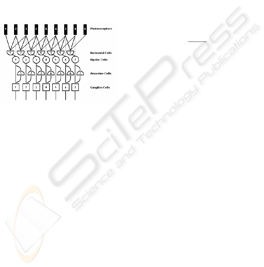
distributed structure. In fig. 1 the digital

representation of all five retinal cells and their

interconnections is shown.

Figure 1: Digital representation of the retinal layers.

All retinal cells can be divided into two

processing layers by their functionality. The first

layer is presented by the photoreceptors, horizontal

and bipolar cells, and performs the edge extraction

(Hubel, 1995), (Olveczky et al., 2003), while the

second layer, which is formed by the amacrine and

ganglion cells, performs among other tasks the local

motion detection and the direction of movement

estimation (Masland, 2001), (Berry II et al., 1999).

Since the contrast adaptation also begins in the

lower retinal layers (amacrine and ganglion cells), it

is important to understand the responses from the

higher processing layers (photoreceptors – bipolars).

2.2 Modelling of the Bipolar Cells

Response

The processing on the first layers starts from

photoreceptors that sense the incoming light. Some

of the photoreceptors are activated by the presence

of light while others are activated when they do not

detect light. All of them are arranged in a circular

way so that one type is surrounded by other types

(center–surround organization). In this paper we use

the ‘on–center’ surrounding organization scheme

(Hubel, 1995).

On the next level, the horizontal cells get their

input from the photoreceptors. They play a very

important role in reducing the amount of information

that is given to the inner brain and represent an

additional mechanism which helps to adjust the

retina response to the overall level of illumination.

Their task is to measure the illumination across a

broad region of photoreceptors and pass the average

value further to the next level. Such calculation can

be represented by Equation 1, where P

is the output

of each photoreceptor that is connected to a

horizontal cell H

; n is the number of inputs of a

certain horizontal cell.

∑

(1)

On the third level, the bipolar cells get their

inputs from the center photoreceptors directly and

from the surrounding photoreceptors indirectly

through the horizontal cells. These two inputs build

the receptive field of each bipolar cell.

The function of the bipolar cell involves a

subtraction mechanism: it subtracts the value of the

horizontal cell H from the value which is received

from the center photoreceptors. Thus, the output of

each bipolar cell B

can be represented by the

Equation 2, where B

is the input from the

photoreceptors and the B

– is the input from the

horizontal cell H

= B

– B

(2)

The output of each bipolar cell forms the

response from the whole receptive field and in this

stage retina performs the edge extraction function

(Olveczky et al., 2003). As it is known from the

classical theory for image processing (Shapiro,

2001), the edge detection operators highlight the

boundaries between regions of different intensities.

This is, naturally, how human beings perceive the

perimeter of an object, when it differs by its

intensity from the background. In fig. 2 the stimuli

with a step-change border and a simplified model of

the first stages of the retina are presented. Here we

assume that each photoreceptor corresponds to a

single pixel in the image and each bipolar cell B is

driven by the receptive field which is constructed by

three photoreceptors – one for the center response

and two for the surrounding. The receptive fields of

the different bipolar cells overlap each other (Hubel,

1995) and, thus, each photoreceptor is fed not only

to the single bipolar cell, but to a number of bipolar

cells.

BIOSIGNALS 2008 - International Conference on Bio-inspired Systems and Signal Processing

514

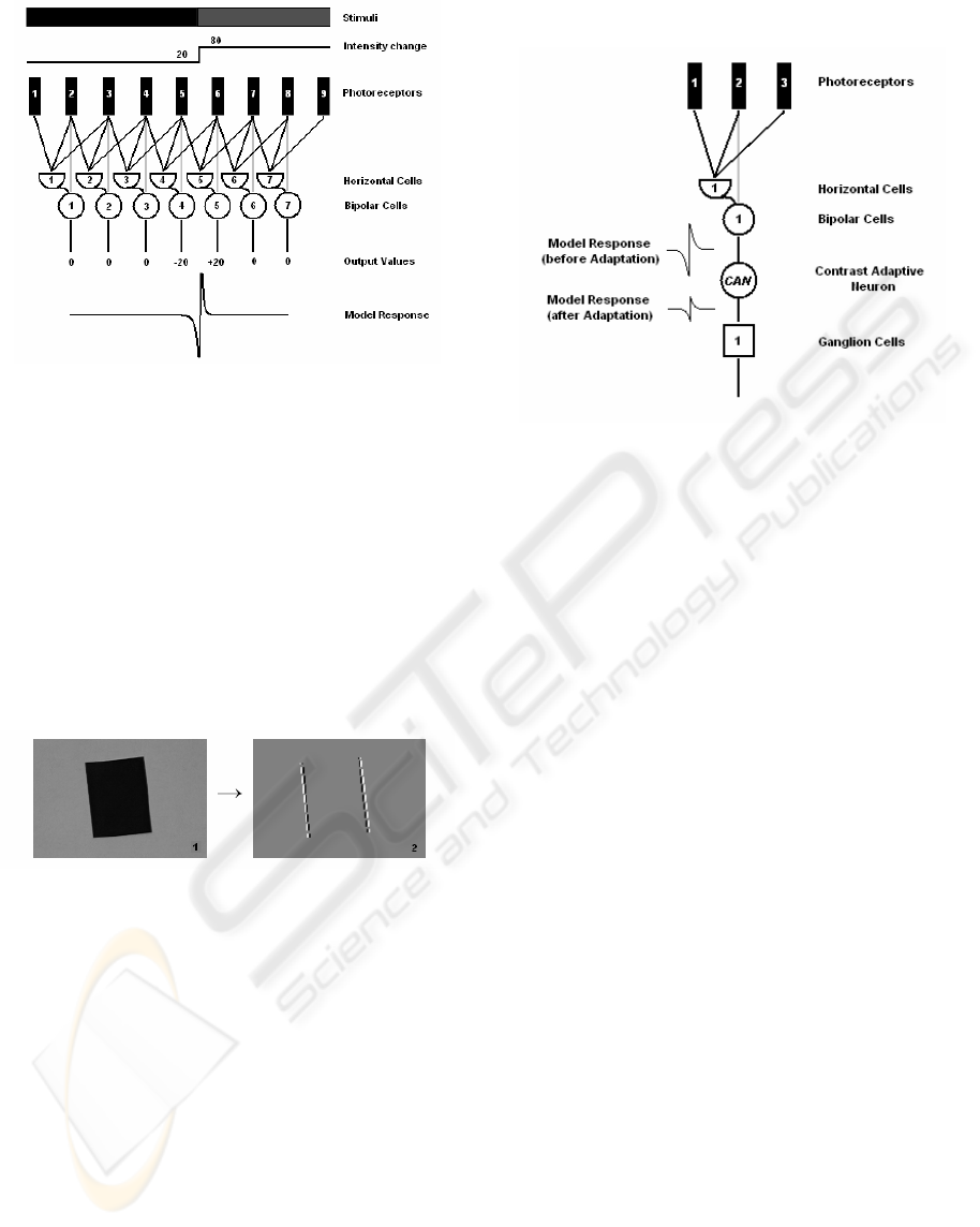
Figure 2: The model and its edge response.

In this example the stimuli change their

intensities between the receptors 5 and 6 from 20 to

80. The model’s response on the step-change border

can be presented by the activities of the two peaks

(negative and positive) exactly at the border between

the two regions. The absolute values of the peaks are

equal, but differ by the sign. Such bio-inspired edge

extraction technique called zero-crossing has been

confirmed by Marr (Marr, 1982) while investigating

the neurobiological background of vision. Fig. 3

shows the response of the bipolar cells at vertical

edges.

Figure 3: The stimuli and the bipolar cell’s response at

vertical edges.

The bipolar cells are fed to the amacrine and

ganglion cells, but first the signal from the bipolar

cell reaches the Contrast Adaptive Neuron.

2.3 Contrast Adaptive Neuron and its

Function

According to (Smirnakis et al., 1997), when the

mean intensity of ambient light increases, the retina

becomes less sensitive. This process is organized

with the help of the contrast adaptive neuron (CAN),

which is located just after the bipolar cells and

serves to adjust the input activity of the ganglion

cells in order to use their dynamic range more

efficiently. In fig. 4 the simplified model of the

receptive field for a single ‘on–center’ ganglion cell

with a CAN is presented.

Figure 4: The model of the ganglion cells receptive field

with CAN.

For fig. 4 we assume that the response generated

by the bipolar cell lies above the ganglion cells

dynamic range and the CAN brings the bipolar cell

response back to the dynamic range of the ganglion

cell by changing its amplitude value. However, the

retina adapts the high and low intensities differently.

When the contrast changes from low to high

(positive contrast change, e.g., going from normal

light room conditions to the strong sun light at

midday), in the first tens of a second the retina

decreases the sensitivity of CAN dramatically, that

results in a quick decrease of the ganglion cell’s

activity. Such first step of the adaptation process is

called “Fast adaptation” and helps to bring the

ganglion cell input nearly to its normal input range.

After that the second “Slow adaptation” phase

occurs and lasts for about ten-fifteen seconds. Its

main task is to fine tune the input of the ganglion

cell and bring it completely to the middle point of

the ganglion cell’s dynamic range.

In case, when the contrast changes from high to

low (negative contrast change, e.g., going from sun

light to the room with normal light conditions), the

retina reacts differently. There is no fast adaptation

process, but the retina increases step-by-step the

sensitivity of the ganglion cells by scaling up their

inputs (with help of CAN). It takes up to twenty-

twenty five seconds till the inputs of the ganglion

cells are in their dynamic range.

These two statements were confirmed by

Solomon et al (Solomon et al., 2004) while

observing the reaction of the isolated retina of a tiger

salamander during contrast changes. Fig. 5 shows

the adaptation process for negative and positive

contrast changes.

A BIO-INSPIRED CONTRAST ADAPTATION MODEL AND ITS APPLICATION FOR AUTOMATIC LANE MARKS

DETECTION

515

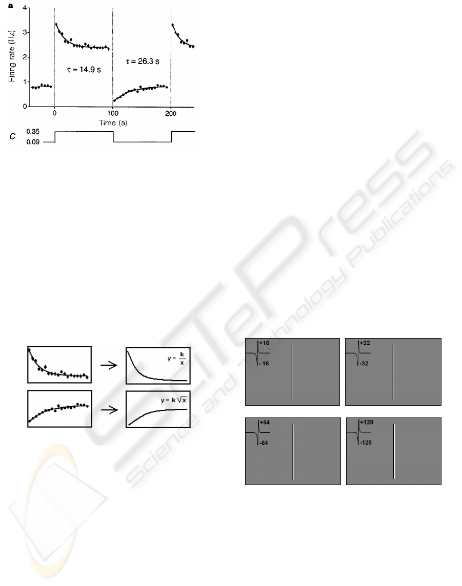
Figure 5: Contrast adaptation in salamander’s retina from

(Solomon et al., 2004).

In fig. 5 C depicts the contrast change values

while the graphical representation shows the

adaptation in the Salamanders retina on different

contrast changes.

We investigated which functions might

approximate the curves for “negative” and

”positive” adaptation and found out that for the

approximation of the “positive” contrast adaptation

process (fig. 6a, upper image) a simple rational

function (fig. 6b, upper image) can be used.

“Negative” contrast adaptation curve (fig. 6a, lower

image) can be approximated by the square root

function, which is shown in fig. 6b (lower image).

a) b)

Figure 6: a) Natural adaptation curves (from (Solomon et

al., 2004)) and b) their approximation functions.

Here, in both functions the coefficient k is a

scaling factor, which is responsible for the CAN’s

selectivity. It controls how strong the adaptation

should be in order to make the ganglion cells more

or less sensitive, depending on the current light

intensity situation. For instance, when the light

intensity is high (e.g., in sunny midday) than the

CAN should scale the intensity down by setting a

rather large k; however, when the light intensity is

just a bit above the dynamic range, the CAN should

fine tune the contrast by setting a quite small value

for the scaling coefficient. In this work we use the

fuzzy-like sets for the definition of CAN’s selectivity

coefficient k.

3 USING FUZZY-LIKE SETS FOR

CONTRAST ADAPTATION

In recent decades a number of applications were

found for fuzzy logic in economics, mathematics

and engineering. Firstly introduced in (Zadeh, 1965),

it is very helpful for modelling highly nonlinear

processes like natural contrast adaptation

3.1 Definition of a Fuzzy – like Set for

Normal Contrast

For the graphical representation of the model’s

response we should declare, what the Normal

contrast means and create a corresponding fuzzy –

like set for its definition.

Since we are working with bio-inspired edge

extraction based on zero-crossings, we assume here

that the absolute zero, as it shown on the

characteristic curve in fig. 2 will be equal to the

intensity 128, which represents the middle point of

the intensity spectrum. When model analyzes the

border between object and background, on the

graphical representation the response will drop down

and then raise up by a certain value (e.g., dark and

light vertical lines in fig. 3, image 2).

Then we analyzed which intensity differences

can represent the Normal Contrast value (see fig.7).

Figure 7: Biological edges with 16, 32, 64 and 128

intensity difference levels.

Fig. 7 shows four biological edges with

intensities 16, 32, 64 and 128. The edges with the

intensity differences of 16 and 32 do not have

enough contrast and should be adapted. The edges

with intensity difference of 64 and 128 do have

enough contrast and thus there is no need for

adaptation. However, in the real world situation the

biological intensity difference of 128 is hardly

possible, because it causes an intensity change of

255 levels at the object-background border (e.g.,

BIOSIGNALS 2008 - International Conference on Bio-inspired Systems and Signal Processing

516

changing from black to white). Normally the

contrast numbers, which can be detected in real

images, lie in the range from 120 to 200, which

caused the biological edge of [± 60 – ±100] to

appear. That is why we do not have to adapt the high

intensity values (e.g., from 180 to 255), we should

only define such a process, which will adapt the

edge values from the lower part of the intensity

difference spectrum and bring them in to the middle

region. Thus, only the “negative” contrast adaptation

process should be used (fig. 6, lower images).

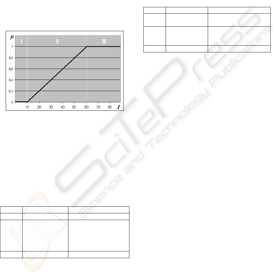
Following this, we introduce a Normal Contrast

fuzzy variable which should adapt all the values that

lie under the intensity 60. It is presented in fig. 8.

Figure 8: Fuzzy variable for Normal Contrast.

On this image, the X-axis represents the intensity

change I on the biological edge and Y-axis shows

the membership μ of a certain intensity value in the

Normal Contrast variable.

There are three characteristic adaptation regions

presented on this graphic. Since the fuzzy logic

operates with linguistic variables, table 1 shows such

a linguistic description and action which is needed

for a certain region.

Table 1: Linguistic definition of the model.

Region Intensity Action needed

I Low Intensity Strong adaptation

II Low–to–Normal

Intensity

Adaptation based on the

μ membership

coefficient in order to

control adaptation

strength

III Normal Intensity No adaptation needed

When the bipolar cells deliver low intensities

(values from 1 to 10), strong adaptation is needed; in

the mid-range (values from 11 and 60), adaptation is

also needed, but the system should control the

strength of the adaptation by using the membership

coefficient μ; and when the intensity is normal

(values above 61), then no adaptation is needed.

In order to create the system we should define

the set of rules for each of the regions

mathematically. Since we are using the “negative”

adaptation process, a curve that will represent this

process should have the shape of the square root

function. Table 2 shows the mathematical

representation for each action regions.

Table 2: Mathematical representation of the model.

Region Intensity values Representation

I 1 – 10 K = 2 ·√x

new

= I

· K

II 11 – 60 μ = (2 · I

+ 20) / 100

K = (2 - μ) · √x

new

= I

· K

III 61 – 127 I

new

= I

The adaptation process in nature lasted for

several seconds. Here this process is modelled with

iteration mechanism and x represents current

iteration; K is an adaptation coefficient and should

be calculated differently for regions I, II and III. It

represents the CAN selectivity and controls the input

gain to the ganglion cells. I

represents the input

intensity of CAN and I

new

is a new calculated value

of the adapted intensity; μ is a membership

coefficient, which influences the amplification factor

and is calculated according to the equation of the

characteristic line in region II (see fig. 8).

3.2 Adaptation Algorithm

The algorithm for the contrast adaptation involves

all the definition for the variables that have been set

early, like I

, I

low

, I

normal

, I

new

, μ, K and x which is

initially set to 0. Firstly, based on the current

intensity I

, μ is calculated.

if (I

>1&&I

<=I

low

){μ = 0}

if (I

low

&&I

<=I

normal

){

μ = (2·I

+20)/100}

if (I

normal

){μ = 1}

Then the adaptation coefficient K and the

adapted intensity I

new

based on the equations in table

2 is calculated.

if (μ<1){

while (I

new

<=I

normal

){

K = (2 - μ) · √x

new

= I

· K

x = x + 1;

}

A BIO-INSPIRED CONTRAST ADAPTATION MODEL AND ITS APPLICATION FOR AUTOMATIC LANE MARKS

DETECTION

517

else {I

new

}

The process stops, when the calculated intensity

new

reaches the normal intensity I

normal

that has been

set to 60 empirically.

3.3 Adaptation Results

During the investigation and development the model

has been tested on different types of images.

Experiments were divided into three categories by

the specific adaptation process:

• adaptation of the low contrast;

• adaptation of the low-to-normal contrast;

• adaptation of the real world images;

The first two categories were tested with

synthetic images. Synthetic images were chosen

because the results of the processing can be

predicted in order to make the model’s proof of

concept under different conditions. To demonstrate

it a number of images with different intensity

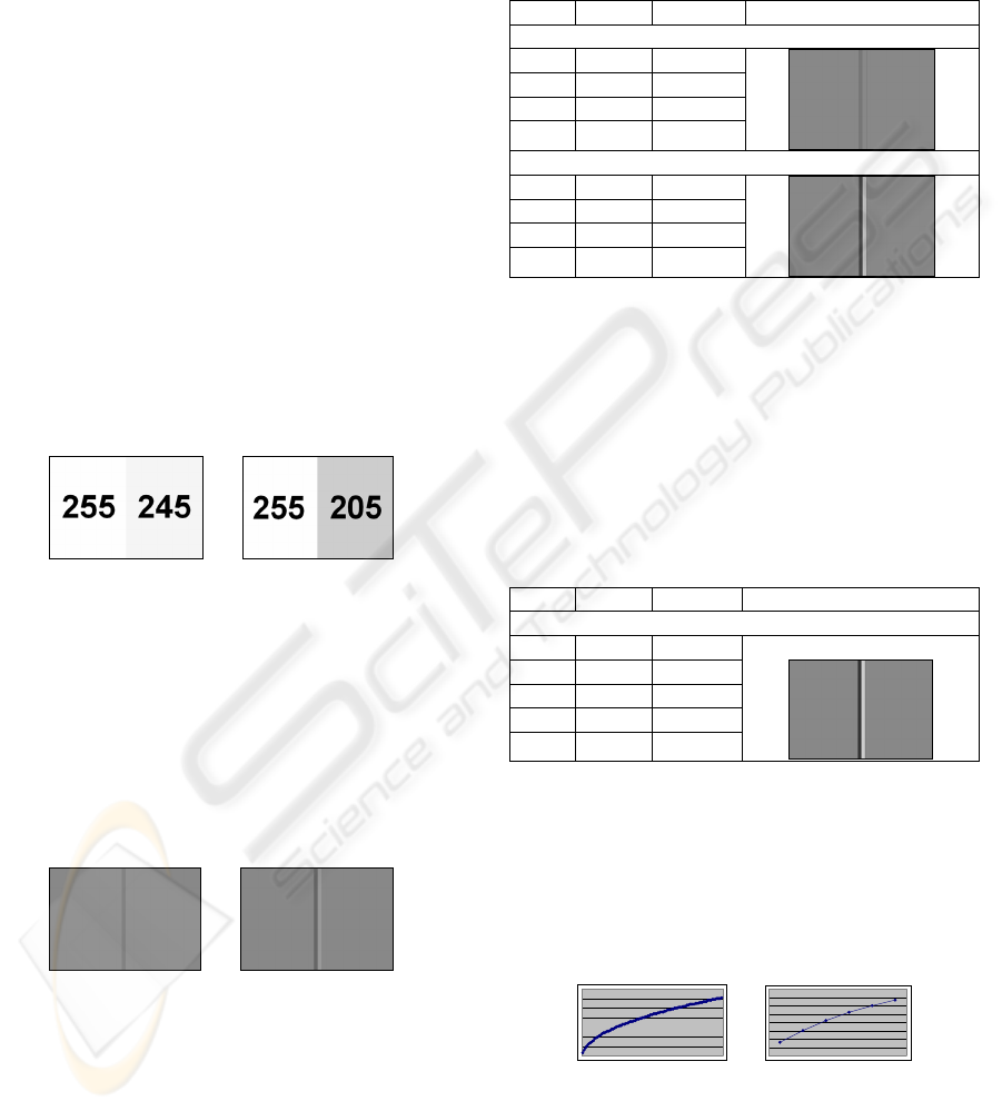
changes were chosen. Fig. 9 represents two of them.

a) b)

Figure 9: Experimental data.

Fig. 9a shows the intensity change of 10 levels

(from 255 to 245) and figure 9b corresponds to a

change of 50 levels (from 255 to 205) of the

intensity spectrum. The digits on the images

represent just the absolute intensities and will not

appear in the modelling results.

Fig. 10 shows the calculated bipolar cells

activity for fig. 9a and 9b correspondently.

a) b)

Figure 10: Calculated bipolar cell’s responses to the

experimental data in fig. 9.

For the first experiment we took fig. 10a. The

initial data (fig. 9a) shows minor intensity change at

the object-background border, which causes a low

contrast and hardly distinguished border response

(fig. 10a). The initial intensity change I

equals 3

(see equations 1 and 2), which corresponds to the

low intensity region in fig. 8. Initial data: I

= 3; μ =

0, => K = 2 ·√x.

For the adaptation of such a low intensity 104

iterations are needed. Table 3 shows some of them.

Table 3: First experiment data.

x K I

new

Graphical representation

1 2 6

2 2.82 8

3 3.46 10

4 4 12

…

101 20.09 60

102 20.19 60

103 20.30 60

104 20.40 61

The second experiment has been performed with

fig. 10b. The initial intensity change here I

is 16,

which corresponds to the low-to-normal intensity

region in fig. 8. Adaptation is still needed, but the

strength of the adaptation should be controlled.

Initial data: I

= 16; μ = 0.12, => K = (2 - μ) · √x.

According to the algorithm, the adaptation of

such intensity will be done in 5 iteration steps. Table

4 represents this process.

Table 4: Third experiment data.

x K I

new

Graphical representation

1 1.88 30

2 2.65 42

3 3.25 52

4 3.76 60

5 4.20 67

x = 5, I

new

= 67:

As it can be seen on the results presented above,

the contrast adaptation model shows the expected

responses on the different stimuli with different

adaptation time. The intensity change adaptation

correlates with its natural representation (fig. 6,

lower image). To confirm this, fig. 11 shows the

adaptation curves for each experiment.

a) b)

Figure 11: Adaptation curves for all experiments.

BIOSIGNALS 2008 - International Conference on Bio-inspired Systems and Signal Processing

518

3.4 Adaptation of the Real World

Images

The model has been already tested on the synthetic

images; the next step is to see how it will respond on

the real world images. For this purpose we choose a

number of images with the real road scenes that have

been taken on a german highway. Some of these test

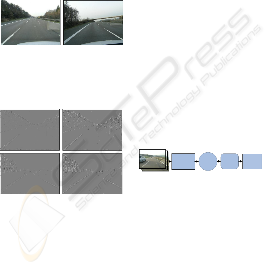
images are shown in Fig. 12.

Figure 12: Real road scenes.

Then we processed the images first with the

classical biological edge operator without the

contrast adaptation mechanism. On the 2

phase the

same images have been processed with the bio-

inspired edge operator and with the contrast

adaptation module. Fig. 13 shows the results.

Figure 13: Calculated biological edge without (left) and

with (right) contrast adaptation for fig. 12.

The difference between the adapted and the not

adapted images can be clearly seen. The edges, that

are even not fully visible on the left images, are well

seen on the right ones. Besides, the initial images

(fig. 12) were taken under slightly different

illumination conditions: the first image was taken

under bright sun light while the second one at early

evening. Nevertheless, the adapted images show

good results especially in underlining the lane road

marks. This gives the possibility to use this contrast

adaptation model for robust lane detection.

4 LANE DETECTION

APPLICATION

Lane keeping assistant systems have been described

in a number of recent publications, e.g. (Risack et

al., 2000), (Chang et al., 2003). For such systems

detection of the lane marks is a key feature for

further processing. The lane marks form lines with

certain slopes and thus, for its detection a good

shape extraction method is needed.

The Hough transformation (Leavers, 1992) is a

pattern recognition technique which is known for its

performance in locating given shapes in images.

Some researches have reported that the Hough

transform correlates with the processes that happen

in the striate cortex and in fact, reproduces the

natural mechanism of objects contour extraction

(Hubel, 1995), (Blasdel, 1992), (Ballard et al.,

1983), (Brueckmann et al., 2004).

Very interesting state-of-the-art research work is

presented in (Serre, 2007). The authors describe the

usage of the midbrain biological mechanisms for the

real world scene segmentation and objects

recognition. Furthermore, they also use the Hough

transformation as a shape localization method.

That is why we propose to use the Hough

transform as a lane marks detection method together

with the retina model with contrast adaptation as a

preprocessing method. This gives the possibility to

create a fully bio-inspired system for the lane mark

detection. The architecture of such a system is

shown in fig. 14.

Image

Acquisition

& Biological

Edge Detection

Hough

Processing

Contrast

Adaptation

Results

Interpretation

Road Image Sequences

Figure 14: Architecture of the bio-inspired lane detection

system.

The biological edge detection and contrast

adaptation stages were well described above. In fig.

14, after contrast adaptation the Hough

transformation takes place. Hough transformation

involves a voting scheme for the shape detection. In

particular, here we extract the lines of the different

slopes. Fig. 15 represents the Hough spaces built

from road edge picture (fig. 13, two right images)

and then the maximas are marked.

A BIO-INSPIRED CONTRAST ADAPTATION MODEL AND ITS APPLICATION FOR AUTOMATIC LANE MARKS

DETECTION

519

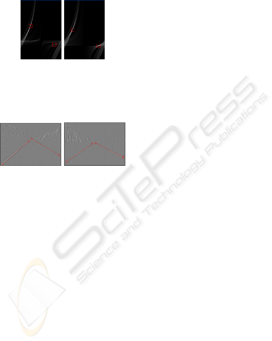
Figure 15: Hough spaces with local maximas.

After the maxima were detected, the

interpretation of the results should be performed.

Each maximum on the Hough space corresponds to

the line with a certain slope in a Cartesian space and

after processing the detected lane marks will be

highlighted. Fig. 16 shows the final results.

Figure 16: Detected lane marks in the adapted images.

5 CONCLUSIONS AND FUTURE

WORK

In this paper a bio-inspired model for contrast

adaptation has been presented. The model has been

tested with different test sets and showed good

results. Furthermore, the proposed contrast

adaptation algorithm has been coupled with the

Hough-based lane marks detector. This coupling

showed good performance and full correspondence

to the predicted behaviour.

Future work will concentrate on development of

the lane keeping assistant system using the bio-

inspired techniques further. In particular, for the

preprocessing stage the colour perception model will

be investigated, implemented and will be used for

the road scenes segmentation and traffic signs

detection.

Besides, for the post-processing and trajectory

prediction stages time-to-lane crossing approach will

be taken in to the account. It is likely possible that it

might be modelled with the natural timing delay-

computational maps. This problem will be also

investigated and the results will be reported.

REFERENCES

David H. Hubel, Eye, Brain and Vision, Freeman, 1995.

Linda G. Shapiro, George C. Stockman, Computer Vision,

Prentice-Hall , 2001.

Bence P. Ölveczky, Stephen A. Baccus & Markus Meister,

“Segregation of the object and background motion in

the retina,” Nature, Vol. 423, May 2003, pp. 401 –

408.

Richard H. Masland, “The fundamental plan of the

Retina,” Nature Neuroscience, Vol.4 No. 9, September

2001, pp. 877 – 886.

Michael J. Berry II, Iman H. Brivanlou, Thomas A. Jordan

& Markus Meister, “Anticipation of moving stimuli by

the retina,“ Nature, Vol. 398,March 1999, pp. 334–

338.

Hugh R. Wilson, “Nonlinear processes in the visual

discrimination”, Proc. Natl. Acad. Sci. USA, Vol. 90,

1993, pp. 9785 – 9790.

Stelios M. Smirnakis, Michael J. Berry, David K.

Warland, William Blalek & Markus Meister,

“Adaptation of retinal processing to image contrast

and spatial scale,” Nature, Vol. 386,March 1997,pp.

69–73

Stephan A. Baccus & Markus Meister, “Retina Versus

Cortex: Contrast Adaptation in Parallel Visual

Pathways”, Neuron, 2003, pp. 5 – 7.

Stephan A. Baccus & Markus Meister, “Fast and Slow

Contrast Adaptation in Retinal Circuitry,” Neuron,

Vol. 36, 2002, pp. 909 – 919.

Samuel Solomon, Jonathan Peirce, Neel Dhruv, Peter

Lennie, “Profound Contrast Adaptation Early in the

Visual Pathway”, Neuron, vol. 42, 2004, pp. 155–162

Zadeh L.A., “Fuzzy Sets”, Information and Control, 1965,

vol. 8, pp. 338 - 353.

Marr D., Vision, Freeman, pp. 54 – 78. 1982.

Risack, R.; Mohler, N.; Enkelmann, W., A video-based

lane keeping assistant, Intelligent Vehicles

Symposium, 2000. Proceedings of the IEEE, pp. 356 –

361, 2000.

Tang-Hsien Chang; Chun-Hung Lin; Chih-Sheng Hsu;

Yao-Jan Wu. A vision-based vehicle behavior

monitoring and warning system

Proceedings IEEE, Volume 1, pp. 448 – 453, 2003.

Leavers, V.F., Shape detection in Computer Vision using

Hough Transform. Springer – Verlag, p.201, 1992.

Gary G. Blasdel, “Orientation Selectivity, Preference, and

Continuity in Monkey Striate Cortex”, The Journal of

Neuroscience, Aug. 1992, 12 (8): 3139 – 3161.

Ballard D., Hinton J., Sejnowski T., Parallel visual

computation. Nature 306, pp. 21 – 26, 1983.

T. Serre, L. Wolf, S. Bileschi, M. Riesenhuber, and T.

Poggio, “Robust Object Recognition with Cortex-like

Mechanisms”, IEEE Trans. on Pattern Analysis and

Machine Intelligence, vol. 29, no. 3, March 2007.

Brueckmann, A., Klefenz F., Wuensche, A. A neural Net

for 2-D Slope and Sinusoidal Shape Detection.

International Scientific Journal of Computing. Vol. 3

(1), pp. 21 – 26, 2004.

BIOSIGNALS 2008 - International Conference on Bio-inspired Systems and Signal Processing

520