EFFICIENT PLACEMENT OF WIRELESS BASE-STATIONS IN

URB

AN ENVIRONMENT

Mansour A. Aldajani

Center for Communications and Computer Research, KFUPM, Dhahran, Saudi Arabia

eywords:

Wireless Communications, Cell planning, Base Station, Placement, Convolution.

Abstract:

This work proposes a novel approach for placing wireless base-stations in urban environments. The new

approach solves the placement problem using 2-D convolution. Convolution searches for the best locations of

base stations based on highest consumption criteria. Convolution theorem is then used to substantially cut the

computation load of the proposed approach. The approach allows simple user-interface and arbitrary demand

and supply patterns of power. Simulations show that the new approach can be used to efﬁciently model and

place wireless base-stations.

1 INTRODUCTION

Placing wireless base-stations is a complex process

which usually involves many parameters and requires

long time to solve. Modeling the placement problem

using conventional optimization techniques is com-

plex and need expert knowledge of the considered

technique. Moreover, the solution approach usually

take long time for moderate grid-size resolution.

One of the ﬁrst studies to solve the placement

problem was in (Sherali and Rappaport, 1996). In

this study, the solution of single as well as multiple

transmitters problem was considered. The problem

was modeled as a nonlinear program and then three

nonlinear optimization algorithms were considered to

solve this model. The work in (Hao Q., 1997) for-

mulated the placement problem as a large-scale com-

binatorial optimization model. The model is then

solved using the simulated-annealing approach. The

Hata’s propagation model (Hata, 1980) was used to

determine the transmission loss in this study. Similar

model was developed in (Calegari, 1997). The model

in this work was solved using generic algorithms re-

sulting in sub-optimal solutions. The work in (Park

and Park, 2002) considered the determination of both

BSs placement as well as transmission power. A sim-

ple weighted objective function was established. The

real-coded generic algorithm was then used to obtain

the solution. The solution takes into account the inter-

ference situation to determine the appropriate trans-

mission power. Transmission power in wireless sys-

tems can also be adjusted via well-developed power

control techniques (Aldajani and Sayed, 2003).

In this work, we present a new approach for plac-

ing wireless base stations in urban environment. The

approach uses convolution as a core process to come

up with a minimum number of base-stations such that

the minimum coverage level is achieved. Fast algo-

rithms for computing the convolution are then used to

substantially reduce the computation load.

2 PROBLEM FORMULATION

The objective of the placement problem is to mini-

mize the total number of base-stations N such that the

net power inside a 2-D Euclidian space Γ is at least

equal to the power threshold α at all locations. In

other words,

p(x, y) ≥ α ∀ x, y ∈ Γ (1)

where p(x, y) is the net power at the point with coor-

dinates (x, y).

To ﬁnd an expression for p(x, y), let us deﬁne the

quantity s

(x, y) as the power supplied by the n

to the mobile station at location (x, y). This quantity

A. Aldajani M. (2007).

EFFICIENT PLACEMENT OF WIRELESS BASE-STATIONS IN URBAN ENVIRONMENT.

In Proceedings of the Second International Conference on Wireless Information Networks and Systems, pages 33-38

DOI: 10.5220/0002145200330038

 SciTePress

indicates simply the signal strength at location (x, y)

due to station n. This quantity is dependent mainly on

the radio propagation and path loss model of the trans-

mitter antenna. For example, for omni-directional an-

tenna in free-space, the quantity s

(x, y) is given by

the well-known Friis equation (Janaswamy, 2000)

(x, y) =



4πh

(x, y)



(2)

where

, G

, and λ are the transmission power,

transmitter gain, receiver gain, and wave length re-

spectively. h

(x, y) is the distance between the point

(x, y) and the base-station n.

Let us also introduce the term d(x, y) to represent

the demand level at point (x, y). This quantity can

be used to model different priorities of coverage and

extra signal attenuations at location (x, y).

Then we can deﬁne the net power p at location

(x, y) as follows

p(x, y) = max

n=[1,N]

(x, y)} − d(x, y). (3)

We assume here that the mobile station at location

(x, y) will connect to the base station that delivers the

maximum signal power.

The objective of the placement problem is to ﬁnd

the minimum number of base-stations and their loca-

tions that will satisfy the power constraint (1) where

p(x, y) is given by (3).

2.1 Discretization of the Model

The variables p(x, y), s

(x, y), and d(x, y) are dis-

cretized in 2-D Euclidian space to form the matrices

P, S

, and D respectively. Therefore, the optimization

problem can be written in matrix format as

min N (4)

subject to

= max

n=[1,N]

} − D ≥ α (5)

where P

is the power pattern matrix of size (I × J)

after assigning N base-stations, S

is the power sup-

ply matrix of the n

BS, and D is the demand pattern

matrix. Notice that this constraint states that all the

elements of the matrix P

should be greater than the

power threshold α.

The matrix S

can be broken down into the convo-

lution of two matrices as follows

= X

⊗ A (6)

where the symbol ⊗ indicates the 2-dimensional con-

volution. The matrix A of size (I

× J

) is a ﬁxed

propagation pattern matrix of the transmitter radio an-

tenna. The matrix X

indicates the location of base-

station n. If we denote this location by the coordinates

, v

) then X

has all its elements equal to zero ex-

cept at (u

, v

) where it equals to “1”. In other words,

(i, j) =

(

1 at (u

, v

)

0 elsewhere.

(7)

Expression (6) means simply shifting the elements of

the A matrix by (u

, v

Notice that minimizing the number of base-

stations N is equivalent to minimizing the summation

norm of the location matrices X

for all base-stations.

In view of this fact, the optimization problem can ﬁ-

nally be written as

min k

∑

n=1

k (8)

subject to

= max

n=[1,N]

⊗ A} − D ≥ α. (9)

3 SOLUTION OF THE

PLACEMENT PROBLEM

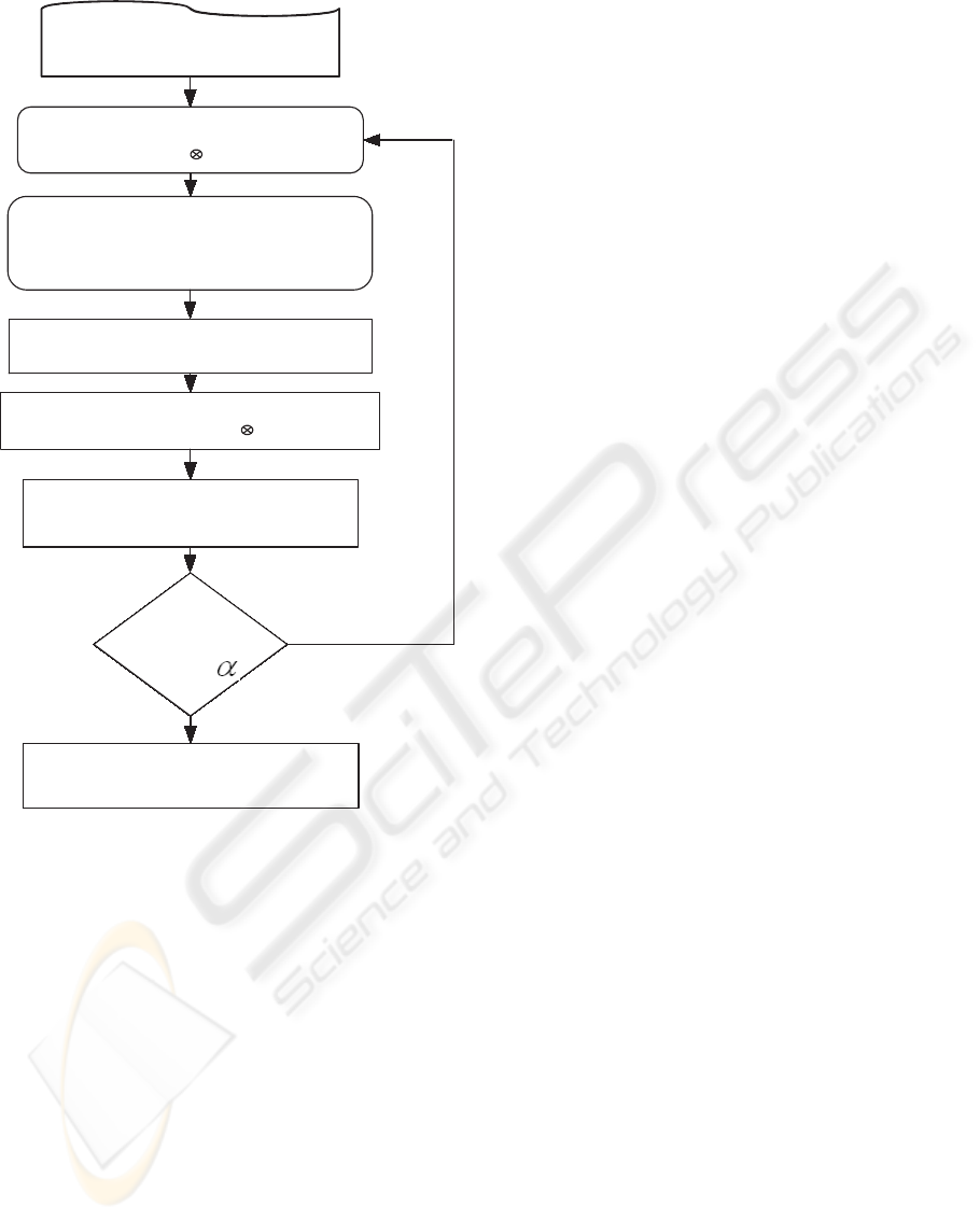
A ﬂow chart of the proposed algorithm is shown in

Fig. 1. To determine the amount of power consump-

tions associated with placing a BS at a certain grid

point, the antenna propagation matrix A is convolved

with the existing power pattern P

n−1

that resulted

from previously assigned BSs, i.e.,

= A⊗ P

n−1

= −D. (10)

The role of the convolution here is as follows. For

each point on the current power pattern P

n−1

, the an-

tenna propagation A is centered at that point and dot-

multiplied with the intersecting sector of P

n−1

. The

multiplication values are then summed up and the an-

swer is stored at the corresponding point in Y

. This

convolution process is repeated for all other points in

n−1

The coordinates that correspond to the minimum

value of the matrix Y

indicates the highest consump-

tion. This point is chosen as the location of the n

base-station,

, v

) = argmin

(i, j)

. (11)

Once a new base-station location is chosen, the lo-

cation matrix X

is constructed from (7). The power

matrix is then updated as follows

= G

− D, n = 1, 2, ...., N. (12)

WINSYS 2007 - International Conference on Wireless Information Networks and Systems

Given A and D

Set n=1, P

0

= -D , and G

0

=0

Calculate the power contributions

Y

n

=A P

n-1

Place the n

th

BS at the minimum

value of

Y

n

;

(u

n

,v

n

)=

argmin

{Y

n

}

Compute the net power

P

n

= G

n

- D

All area

covered?

p

min

(

n) >

Return N, Locations: { u,v }, and p

min

YES

NO

Construct the location matrix X

n

X

n

(i,j ) = 1 at (u

n

,v

n

) and 0 Elsewhere

n=n+1

N=n

Compute the accumulated power

G

n

=max{ G

n-1

, A X

n

}

Figure 1: The proposed solution algorithm.

where G

is the power pattern supplied by the stations

1 to n. This matrix can be computed iteratively from

= max {G

n−1

, S

} = max {G

n−1

, A⊗X

}, G

= 0

(13)

3.1 Penalizing Boundaries of the

Demand Grid

Since the design space is always provided as a con-

ﬁned rectangular region, the demand matrix D need to

be surrounded by a negative frame value w as shown

in Fig. 2 to penalize the boundaries of the grid. The

purpose of the penalty w is to push the locations of

the BSs inward and therefore increase the coverage

efﬁciency. In case of a tie, the algorithm will pick the

value that results in higher p

min

. In this way, not only

the number of stations will be minimized but also the

minimum power will be maximized reﬂecting an im-

proved over-all coverage.

D =







w w w w w w w

w −5 −5 0 0 0 w

w −5 0 +10 +10 +5 w

w 0 0 +10 +10 +5 w

w w w w w w w







Figure 2: Numerical example of the demand matrix D sur-

rounded by the penalty frame value w.

3.2 Veriﬁcation of the Solution

Since analytical solution for the placement problem

given by (8) and (9) is not available, we follow two

numerical approaches to verify the proposed solution.

First, the algorithm is implemented on simple models

where solutions are known and the results are then

compared (Park and Park, 2002). Second, solution

is veriﬁed by performing an exhaustive search on all

possible locations.

4 SIMULATIONS

Matlab was used to implement the algorithm on a

2.1GHz personal computer with 256MB of memory.

The Matlab program provides a friendly User Inter-

face (UI). It inputs a color-coded map, similar to that

of Fig. 3, in a common image format (JPEG) and then

constructs the corresponding demand pattern matrix

D. It also inputs the propagation pattern matrix A. It

then computes the number of base-stations and their

locations and then shows them on the color-coded im-

age. The program also returns the ﬁnal minimum

power p

min

, and the percentage coverage (PC) of each

assigned base-station.

In our simulations, the size of the matrices D and

A is ﬁxed to 41 × 61 for each (corresponds to 2501

possible locations). Furthermore, the power threshold

is arbitrarily ﬁxed in all simulations to the normalized

value α = 1%.

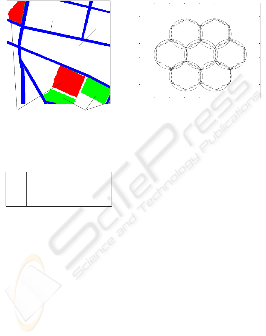
To test the algorithm, we considered the place-

ment problem in (Park and Park, 2002). In this case,

a conﬁguration of seven hexagonal cells is to be cov-

ered with omni-directional antennas having the same

radius as that of the cells. The solution for this prob-

lem is obvious: exactly seven BS are needed which

EFFICIENT PLACEMENT OF WIRELESS BASE-STATIONS IN URBAN ENVIRONMENT

Red: No-Demand

(Avoid)

White: Normal Demand

(Urban area, Campuses, schools, etc.)

Green: Highest Demand

(Malls, Business district,

Large population, etc.)

Blue: High Demand

(Highways, roads, etc.)

Figure 3: Example of designing the demand levels on a real

map using color codes.

Table 1: Example of color codes and their corresponding

values inside the demand matrix D .

Color Demand Value inside D

Green Highest +20

Blue High +10

White Normal 0

Red No− Demand −20

should be located at the centers of the cells. To imple-

ment the proposed approach, the edges of the seven

cells are drawn using popular drawing software and

then feeded directly to the algorithm. The edges are

mapped as negative values in D. The results are

shown in Fig. 4. The algorithm achieved 99.7% cov-

erage in seven iterations. Solving the same problem

with Genetic Algorithm (GA), for example, would

need more than 1000 generations to get the same cov-

erage (Park and Park, 2002). Furthermore, the fact

that the model can be built by simply drawing the cell

boundaries and feeding the drawing to the algorithm

makes the proposed approach much more attractive

when compared to the cumbrous modeling process

demanded by the GA.

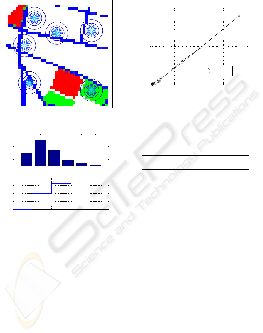
In another experiment, the color-coded map of

Fig. 3 is used in simulation to build a different non-

trivial demand matrix D. The numerical weights as-

signed to the four colors in this example are listed in

Table 1. An omni-directional propagation matrix A

is used here. Fig. 5 shows the resulting placement

0 10 20 30 40 50 60 70 80

Figure 4: Solution of the hexagonal cells problem.

of the base-stations. In this case, six base-stations

were sufﬁcient to meet the coverage requirement. No-

tice that as expected, the ﬁrst base-station was lo-

cated at the green region (corresponds to very high

demand). Also, the algorithm avoided the placement

of any base-station at the red region (correspond to

no-demand region). The minimum power returned by

the algorithm is p

min

= 1.0724 which is just above the

required power threshold α = 1. The optimal frame

value w

∗

in this example is -86. The percentage cover-

age and accumulated percentage coverage for this ex-

ample are shown in Fig. 6. This information can play

very useful role for cell planners. Through this infor-

mation, they have a choice to eliminate those stations

on the map that have negligible coverage. The second

base-station covered about 40% of the area while the

6th one covered about 1% only. This means that if

99% total coverage is sufﬁcient, then the 6th station

can simply be removed. The algorithm returned the

results in less than 2 minutes.

5 COMPUTATION COMPLEXITY

From the discussions above, the proposed scheme has

an outer loop as well as an inner loop. The outer loop

searches for the optimal frame value w

∗

while the in-

ner loop implements Fig. 1 to ﬁnd the location of the

base-stations.

For the outer loop, a simple line search was found

sufﬁcient to ﬁnd w

∗

. The search is limited to the inte-

ger values in the range [w

min

, 0]. Still, more efﬁcient

search algorithm could be adopted to ﬁnd this value.

In the inner loop represented by Fig 1, the only

WINSYS 2007 - International Conference on Wireless Information Networks and Systems

Figure 5: Result of the placement problem with omni-

directional antenna and a given demand map.

1 2 3 4 5 6

PC %

1 2 3 4 5 6

100

APC %

Base−stations

Figure 6: Percentage coverage (PC) and accumulative per-

centage coverage (APC) for the base-stations in Fig. 5.

computationally expensive operation is the convolu-

tion A ⊗ P

n−1

. As mentioned in the motivation sec-

tion, the cost of the convolution can be reduced sub-

stantially from m

to mlog(m) using available fast

convolution techniques (Bernardini and Mian, 1996;

Chiang and Chew, 2005). This feature makes the pro-

posed solution feasible even for large grid-sizes.

Table 2 summarizes the order of complexity for

the proposed approach. In Fig. 7, we show the

simulated and theoretical time needed to assign one

base-station using fast convolution, averaged over 100

runs.

Furthermore, the sparsity of the matrix P

can be

utilized to reduce the computations of the convolu-

tion. This matrix is usually full of zeros. Finally,

the search space reduces as new stations are assigned.

This can also reduce the computation load signiﬁ-

cantly.

0 0.5 1 1.5 2

x 10

0.5

1.5

2.5

Map grid size m=I × J

Time to assign single station (Sec.)

Actual

Theoritical fit

Figure 7: Simulated and theoretical time needed to assign

single station as a function of the grid size m = I × J, us-

ing fast convolution. The theoretical plot is obtained from

βmlog(m), where β is a processing constant.

Table 2: Order of complexity for the proposed approach.

Method used Order of Complexity

for convolution

Direct m

Fast mlog(m)

6 CONCLUSION

In this work, we proposed a new approach for placing

the wireless base-stations. The new approach simpli-

ﬁes modeling and solution of the placement problem.

Modeling the problem is performed by drawing color-

codes on the map. Solution is obtained through the

convolution process which searches for the highest

consumption areas. Convolution theorem is then used

to substantially reduce the computation load. Simula-

tions of the proposed approach showed its efﬁciency

and ﬂexibility in solving the placement problem.

ACKNOWLEDGEMENTS

The author would like to acknowledge the support

of King Fahd University of Petroleum and Minerals,

Dhahran.

REFERENCES

Aldajani, M. A. and Sayed, A. H. (Nov. 2003). Adaptive

predictive power control for the uplink channel in ds-

cdma cellular systems. In IEEE Transactions on Ve-

hicular Technology. Vol. 52, No. 6, pp. 1447 –1462.

EFFICIENT PLACEMENT OF WIRELESS BASE-STATIONS IN URBAN ENVIRONMENT

Bernardini, R., C. G. and Mian, G. A. (Nov. 1996). A new

multidimensional fast convolution algorithm. In IEEE

Transactions on Signal Processing I. Vol. 44, No. 11,

pp. 2853 -2864.

Calegari, P., et al.. (May 1997). Genetic approach to radio

network optimization for mobile systems. In Vehicu-

lar Technology Conference (97). Vol. 2, pp. 755 - 759.

Chiang, I. and Chew, W. C. (July 2005). Fast real-time con-

volution algorithm for microwave multiport networks

with nonlinear terminations. In IEEE Transactions on

Circuits and Systems II: Express Briefs. Vol. 52, No.

7, pp. 370 - 375.

Hao Q., et al.. (Sep. 1997). A low-cost cellular mobile com-

munication system: a hierarchical optimization net-

work resource planning approach. In IEEE Journal

on Selected Areas in Communications. Vol. 15, No. 7,

pp. 1315 - 1326.

Hata, M. (Aug. 1980). Emperical formula for propagation

loss in land mobile radio service. In IEEE Trans. Ve-

hicular Technology. Vol. VT-29, pp. 317-325.

Janaswamy, R. (2000). Radiowave propagation and smart

antennas for wireless communications. Kluwer Aca-

demic Publishing, Massachusetts, USA.

Park, B., Y. J. and Park, H. (Sep. 2002). The determination

of base-station placement and transmit power in an

inhomogeneous trafﬁc distribution for radio network

planning. In Vehicular Technology Conference (02).

Vol. 4, pp. 2051 - 2055.

Sherali, H., P. C. and Rappaport, T. (May 1996). Optimal

location of transmitters for micro-cellular radio com-

munication system design. In IEEE Journal on Se-

lected Areas in Communications. Vol. 14, No. 4, pp.

662 - 673.

WINSYS 2007 - International Conference on Wireless Information Networks and Systems