DIFFUSE MATRIX

An Optimized Data Structure for the Storage and Processing

of Hyperspectral Images

Jose M. Chaves-González, Miguel A. Vega-Rodríguez, Pablo J. Martínez-Cobo

Juan A. Gómez-Pulido and Juan M. Sánchez-Pérez

Univ. Extremadura, Dept. Technologies of Computers and Communications

Escuela Politécnica, Campus Universitario s/n, 10071, Cáceres, Spain

Keywords: Hyperspectral data format, diffuse matrix, storage optimization, geo-rectification, AVIRIS images.

Abstract: This paper proposes a new format for storing and processing hyperspectral images captured by spectrometer

AVIRIS (Airborne Visible/InfraRed Imaging Spectrometer). Obtaining such images is difficult, because the

sensor that takes the images is carried in an aircraft that suffers turbulences while the camera is taking

photos. So, a geo-rectification process is necessary to correct the information of different bands. The format

proposed in this paper, DMF (Diffuse Matrix Format), allows a more efficient storage, because a list with

the original information received in the sensor is saved for each position (X,Y) of the scanned ground. The

format of the list saves space and time because no redundant information is saved using it. To show the

possibilities of this new format an application that makes some thresholding and filter operations has been

built. This program, firstly, creates the diffuse matrix in memory from the file that stores the image

information, and then, some filter operations are executed over the diffuse matrix to check it. In this way,

we prove that diffuse matrix processing is fast and simple, as well as the space used in the disk for its

storage is quite less than the space used by typical formats.

1 INTRODUCTION

Typical raster hyperspectral image formats used in

remote sensing (BSQ, BIL, BIP, HDF-EOS, Geo-

TIFF… (HDF-EOS, 2006)) save redundant

information when they store an image with some

acquisition errors (which is very common).

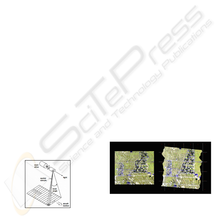
Figure 1: Diagram of hyperspectral image acquisition by

AVIRIS spectrometer.

For this reason, the files that hold such images take

up a lot of space in the hard disk, or at least, more

space than the space necessary. Moreover, the image

processing is not very fast and requires a lot of

memory, because the typical matrix that holds a

hyperspectral image has to be entirely read before

any processing over it.

Figure 2: AVIRIS hyperspectral image before (left) and

after (right) geo-rectification.

The over-information of typical hyperspectral

image formats is caused because the original images,

which are taken using spectrometer AVIRIS

(AVIRIS, 2007) (as it can be seen in figure 1), have

to be pre-processed before any usage with them

(Martínez et al., 2005)(Brunn et al., 2003). This is

M. Chaves-González J., A. Vega-Rodríguez M., J. Martínez-Cobo P., A. Gómez-Pulido J. and M. Sánchez-Pérez J. (2007).

DIFFUSE MATRIX - An Optimized Data Structure for the Storage and Processing of Hyperspectral Images.

In Proceedings of the Second International Conference on Signal Processing and Multimedia Applications, pages 39-44

DOI: 10.5220/0002130800390044

 SciTePress

due to the turbulences suffered by the plane or other

problems that happen while the sensor is taken the

images. Figure 2 shows a hyperspectral image taken

with AVIRIS before and after its geo-rectification.

As we can see in that figure, before rectification, the

image seems to be deformed, because some pixels of

some bands are not in their appropriate place. After

the geo-rectification, the imperfections in the image

are corrected (misplaced pixels are interpolated

using their neighbours).

If we choose an image format that applies geo-

rectification we will have some remarkable

disadvantages, because the process that corrects the

image interpolates the missing or misplaced pixels

with their neighbouring pixels, and this causes that

some information is duplicated, or even erroneous,

in the file that contains the image.

Therefore, the disadvantages of geo-rectification

in the traditional three-dimension formats (Lx,y,l)

carry us to study and develop other ways of

representation, storage and analysis of AVIRIS

hyperspectral images, where any interpolated

information is not saved (so, any redundant or

erroneous information will be not stored in the file).

Some studies to improve hyperspectral data

formats have been published before. It is worth

mentioning Boardman work (Boardman, 1999). He

describes three types of file (IMG, GLT and GEO).

These files are created in the image geo-rectification

process, and they split up the image information

(between data and meta-data information), but this

work is different to ours, because we do not apply

any geo-rectification for the image storage, but when

the image is going to be processed.

The rest of the paper is organized as follows:

section 2 explains the solution suggested in this

work (diffuse matrix), after that we put forward the

application created for this study which works with

the new structure and then, in section 4, we speak

about the obtained results. Finally, conclusions and

future work are expounded in section 5.

2 NEW DATA STRUCTURE:

DIFFUSE MATRIX

There are some criteria that make an image format to

be a good format (Folk, 1998). Between this

characteristics can be pointed out the following:

 The space that it occupies, both in disk and in

memory.

 The easiness of the format (it has to be simple

and easy to understand).

 It has to be self-describing, using a metadata

file or similar.

 Allow sequential access through the image.

 Information access has to be easy to implement.

 Rigorous and perfectly clear definition.

 It has to be efficient: using the format, image

processing algorithms has to run efficiently

and quickly.

We try to follow all the previous requirements in

our work. Besides, we have made a robust format

taking into account the problems caused by the

sensor characteristics (Martínez et al., 2005) (which

are explained in the introduction). Diffuse matrix

separates physical storage and logical processing.

Thus, spectral information is compressed and saved

using a file named DMF (Diffuse Matrix File). In

this file no redundant information is saved, and only

when the structure is loaded in memory (when the

image is going to be processed, but not in its

storage), the required operations to put in order the

spectrum in the matrix are done.

To preserve the acquisition scheme, and to have

the information necessary for each band anytime,

each position in the diffuse matrix (once it is loaded

in memory) is a pointer to a dynamic list, where

each node contains the information shown in fig. 3.

Figure 3: Data register created for each measurement

taken by the sensor.

As it can be seen in figure 3, each register has 6

fields: A pair of fields of two bytes for latitude (Lat.)

and longitude (Lon.) of the scanned area; another

two fields for incidence angle (I.A.) and observation

angle (O.A.); one field of one byte which holds the

pixel spatial resolution (Foot_print size) for the

captured image, and finally, a field of variable

length for the spectrum (data) scanned by the sensor.

In diffuse matrix, each cell contains a pointer,

which points to null if no information is hold for that

coordinate in the matrix (as we said, this structure

saves space, because there are not interpolation of

missing information. If there are nothing, it is saved

nothing); or points to a dynamic list where each

element is a register like the described in fig. 3.

SIGMAP 2007 - International Conference on Signal Processing and Multimedia Applications

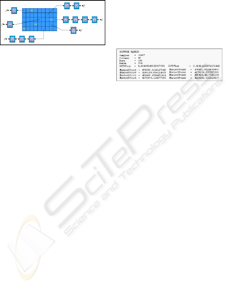
Figure 4: Diffuse matrix structure with some example

nodes (empty and with information nodes).

Figure 4 shows the diffuse matrix structure. At

first sight, the advantages obtained with the usage of

this structure are:

 Diffuse matrix does not need any information

not captured by the sensor, so, any

interpolation or processing is not needed to

save the information.

 Original coordinates (latitude and longitude)

are saved for each measurement.

 Data distribution is independent of

visualization. So, when data are shown, they

have to be organized before, because the

information is saved in an optimal way,

without considering data spatial location.

(Only in the latest stages of data processing,

the interpolation of the image is necessary -to

calculate missing data in the image

acquisition-).

3 AN EXAMPLE OF

APPLICATION FOR DIFFUSE

MATRIX PROCESSING

We have developed a program just to show the

possibilities and the usage of diffuse matrix. The

application fulfils the following goals:

 Diffuse matrix generation from DMF file which

contains it.

 Image visualization using diffuse matrix

structure.

 Performance of some image processing

algorithms over the diffuse matrix (we have

chosen a set of thresholding and filter

operations).

3.1 Diffuse Matrix Loading from DMF

File

A DMF image is divided into two files: a DMF file,

which contains the image, and a HDR file (header

file), which contains meta-information about the

image. Fig. 5 shows the information held in a typical

HDR file. HDR file contains information about the

number of image samples (which will be the number

of cells with information in the diffuse matrix), the

number of rows and columns that the matrix will

have, the number of bands per sample (bands in the

image), and some values to calculate the exact

position (X,Y) of each sample.

Figure 5: HDR file with meta-information about a DMF

image.

To load the diffuse matrix from a DMF file is

necessary to use the HRD file (fig. 5) which is

associated with that DMF file. Loading the image in

the matrix basically consists in reading each sample

sequentially from the DMF file (we know how many

samples there are from HRD file). After reading one

sample, its position is calculated and that sample is

added to the right coordinate in the matrix.

Interpolation will be performed to calculate the final

position of each sample in the matrix if the image is

loaded in memory with some association factor

among the cells. The application allows 4 levels of

association (the user chooses it when the image is

loaded), as we will explain in the following section.

Diffuse matrix structure is hold in memory all

the time while the application is working with the

image. Thus, the position of each sample is only

calculated once at the beginning of the process (not

for every image processing operation), doing it in an

efficient way.

When the process starts, the number of samples

for a particular cell of the matrix is unknown. Only

when the image is completely loaded, we know if in

a particular cell is held one, several or no samples.

So, a matrix of dynamic lists is the best structure to

hold the image in memory.

The position of a particular sample in the diffuse

matrix is obtained using the following equations:

posX=(Lat. - MinLatXPoint) * GIFOVLat

posY=(Lon - MinLonYPoint) * GIFOVLon

(1)

Lat (latitude) and Lon (longitude) values are read

for each sample (fig. 3), while the other values are

the same for all the samples in the image and are

read from HDR file (fig. 5).

DIFFUSE MATRIX - An Optimized Data Structure for the Storage and Processing of Hyperspectral Images

3.2 Image Visualization using Diffuse

Matrix Structure

When the hyperspectral image is shown, it is

considered as a set of n monochrome images (256

grey-levels each). The user chooses the band that

he/she wants to see and this band is shown as a grey

BMP image (in fact, the application allows saving

that image as a BMP image). The user also chooses

the association factor that the matrix cells will suffer

when the image is loaded at the beginning.

Association among cells is allowed because some

cells in the matrix are empty (without samples); so,

if the association is not done, some areas in the

image will not have any information (in this case the

image has some pixels without information, and the

application shows them in purple colour -they are

not processed-). Fig. 6 shows an image loaded with

and without cell association.

Figure 6: Image visualization with no association among

cells (a) and with a 2x2 association (b).

The application allows association factors of 1x1

(no association), 2x2 (groups of 4 cells), 3x3 (groups

of 9 cells) and 4x4 (groups of 16 cells). As we can

see in fig. 6, the more association factor that the

image has, the smaller it appears in the window

when it is shown (this reduction of dimensions has

some performance advantages, as we will see in the

next section). For the right location of each sample

in the matrix, the formulas shown in equation 1 are

divided by the association factor chosen by the user.

For example, the column occupied by a sample is

calculated using the updated formula: posX =

(Latitude - MinLatXPoint) * GIFOVLat /

association factor (the same that in equation 1 but

divided by the association factor).

With the association, it is difficult that any cell of

the matrix stays empty, because in case that the

association factor is, for instance, equal to 2, each

cell contains the samples of 4 neighbouring pixels.

3.3 Image Processing using Diffuse

Matrix

To prove the easiness and potential of diffuse

matrix, we have developed some thresholding and

filter operations (González and Woods, 1992). The

user uses the window shown in figure 7 to configure

the different operations that can be done over the

diffuse matrix.

In this window, the user can configure the band

which he/she wants to work with (on the right area

of the window) and the operation that he/she wants

to apply over the selected band (no operation -only

showing the image-, a thresholding operation or a

filter operation –of smoothing, sharpening or edge

detection-). In particular, we have implemented 15

filters: Average3x3, Average5x5, Average7x7,

Gauss0391, Gauss0625, AverageModA,

AverageModB, Laplace1, Laplace2, SobelX,

SobelY, Sobel45+, Sobel45-, Prewitt1 and Prewitt2.

In summary, we have implemented an important

amount of operations using the structure (both

thresholding operations and convolution operations)

to perform a complete test of the behaviour of the

diffuse matrix for these operations, which are quite

important in image processing. In fig. 8, some

examples of filtering are shown.

Figure 7: Image processing configuration window.

Moreover, if the user chooses association among

the cells of the matrix, an important advantage is

that the image which the application has to operate is

“a dense image”, smaller than the original image, so,

the image processing is faster and more efficient. In

fact, this idea is similar to the one used in Vector

Architectures, with the technique called “scatter-

gather” –which is included on many of the recent

supercomputers–, where data are grouped to process

them faster in a parallel way). In conclusion, diffuse

matrix can be processed faster than traditional

formats if the user chose association among the cells

when the image was loaded.

SIGMAP 2007 - International Conference on Signal Processing and Multimedia Applications

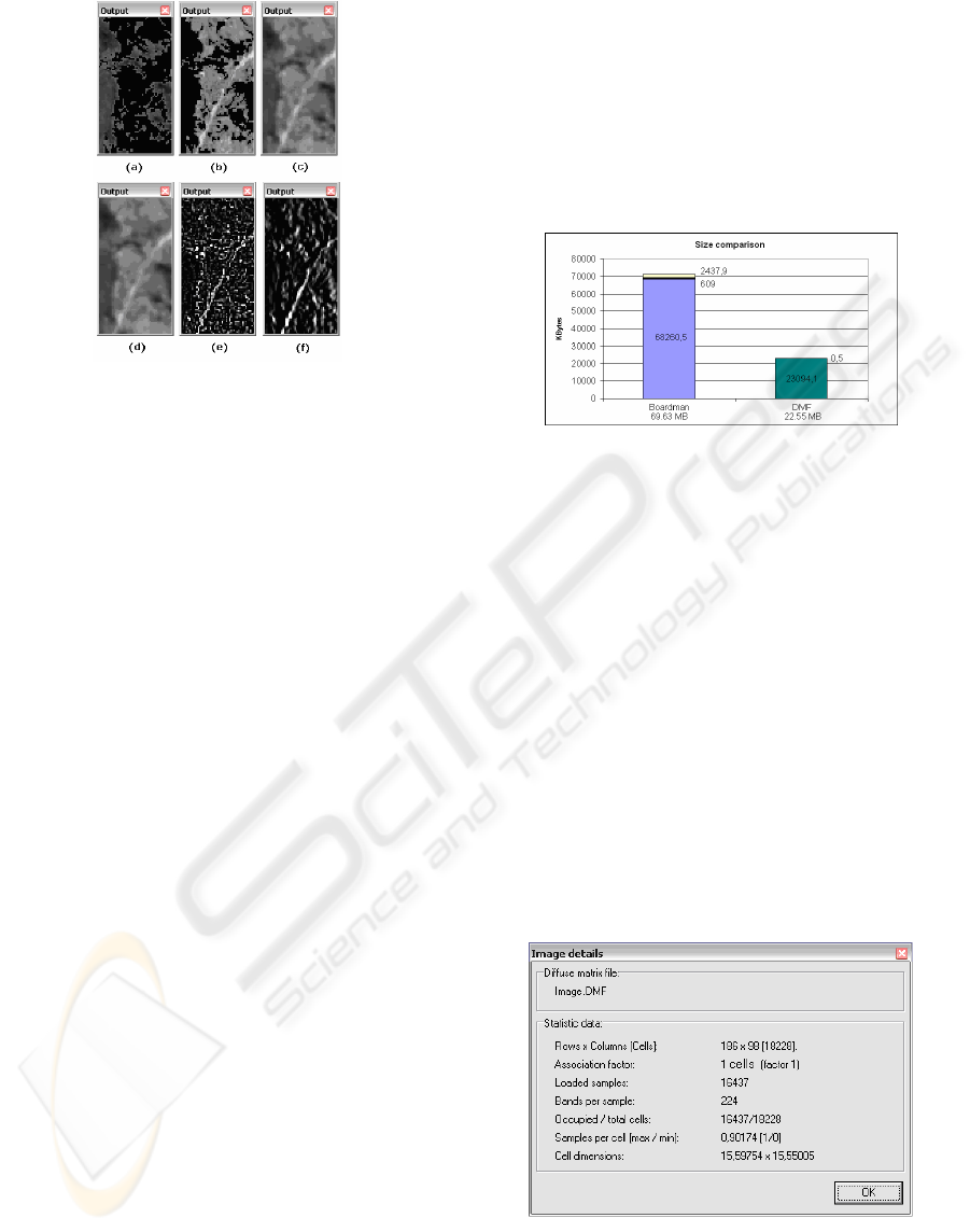
Figure 8: Some example of filters applied over the band 36

of the image.

The filters observed in figure 8 are: (a)

thresholding -pixels with values less than 100

become black-, (b) thresholding -pixels with values

greater than 100 become black-, (c) 3x3 average

filter, (d) Gauss filter, (e) Laplace filter, (f) SobelX

gradient filter.

We have used the following method to

implement every filter operations over the diffuse

matrix: For each cell in the matrix is calculated the

centre position and the distance from this centre to

every sample in the cell. Using these distances, the

weight of each sample over the pixel which is going

to be drawn in that position is calculated. The value

of the pixel associated to a cell is obtained taking

into account all the weights of all the samples in the

cell after a normalization process into the range 0-

255. This process is done for every cell in the

selected band. Finally, the chosen operation is

applied over the normalized pixel matrix and the

result is shown as can be seen in fig. 8.

4 SOME RESULTS OBTAINED

WITH THE STUDY

We have done some size comparisons, and we can

conclude that due to the lack of redundant

information included in the DMF file from geo-

rectification, the size of the image is much smaller

than using traditional formats. In fact, we have done

a comparison with the format proposed by

Boardman in (Boardman, 1999) (which is an

optimization that consist in 3 files to support an

image -GEO, GLT and UTM files-). Using the same

image (IVAHOHA_BEACH_low_altitude), the

following results are obtained: our file with the

diffuse matrix (DMF) occupies 23,648,372 bytes

(22.5 MB) and our HDR file takes up an almost

negligible 551 bytes. On the other hand, the

Boardman solution files take up: 69,898,752 bytes

(66.6 MB) for the GEO file, 624,096 bytes (609 KB)

for the GLT file and 2,496,384 bytes (2.4 MB) for

the UTM file. If we compare the results, the

compression ratio obtained is over 3:1, as we can see

in fig. 9.

Figure 9: Size comparison between Boardman format and

DMF format.

Furthermore, as we said in section 3.2, we can

select an association factor when the image is

loaded. If we associate cells when the matrix is

loaded, the matrix will be compacted in memory (it

has less dimensions) and the final size will be

reduced. In fig. 10 we show the details for the same

image without association factor and in figure 11

with association factor equal to 2. The diffuse matrix

dimensions with an association factor of 2 are

reduced to a quarter, but the cell dimensions are

bigger with the association, because there are more

points for each cell. Moreover, it is important to

point that, as it can be seen in figures 10 and 11,

with no association, the matrix has 0.9 samples per

cell (there was cells with no samples), and with the

association, there are 3.6 samples for each cell (at

least 1 sample per cell and no more than 4 samples).

Figure 10: Image details for an image loaded without any

cell association.

DIFFUSE MATRIX - An Optimized Data Structure for the Storage and Processing of Hyperspectral Images

Figure 11: Image details for an image loaded with cell

association (4 cells).

Anyway, with any association factor, the image

is processed in the same way, because the structure

of the matrix is always the same: a matrix of lists,

where each node in the list contains the information

of a sample acquired by the sensor, with altitude and

longitude data (fig. 3), so the processing of this

structure is homogeneous and efficient.

5 CONCLUSIONS AND FUTURE

WORK

We have described a new format to work with

AVIRIS hyperspectral images. With the DMF

format, the physical storage in the disk (DMF and

HDR files) and the later image processing (diffuse

matrix with or without association of cells) have

been clearly separated. This means that the same

images take much less space in hard disk using DMF

format than other typical formats. Furthermore, the

image can be processed in a more efficient way,

because it is loaded as a matrix of dynamic lists,

taking advantage of the structure used. We have

mentioned some of these advantages in the previous

sections, but moreover, the diffuse matrix makes

easier the parallelization of algorithms, because

when the image is going to be processed, each cell is

independent of the others in the matrix, and it is

possible to divide the diffuse matrix and process

each piece in a separate/parallel way, improving and

speeding up the image processing (this aspect is very

interesting because the size of hyperspectral images

is quite big).

In conclusion, this work is a first step (the most

important milestone) for the upcoming works in next

months. Future work includes: (a) a detailed

statistical comparison among different algorithms

and different formats to get the concrete

improvement obtained by the diffuse matrix in each

case; (b) a study in depth about the parallelization of

some algorithms using the proposed structure

(diffuse matrix).

ACKNOWLEDGEMENTS

This work has been developed in part thanks to the

OPLINK project (TIN2005-08818-C04-03).

REFERENCES

AVIRIS, Jet Propulsion Laboratory, NASA. AVIRIS,

http://aviris.jpl.nasa.gov/, 2007.

Boardman, J.W.. Precision Geocoding of Low-Altitude

AVIRIS Data: Lessons Learned in 1998. 8

Annual

JPL Airborne Geoscience Workshop, Pasadena,

California, USA, 1999.

Brunn, A., Fischer, C., Dittmann, C., Richter, R.. Quality

Assessment, Atmospheric and Geometric Correction of

Airborne Hyperspectral HyMap Data. 3

EARSeL

Workshop on Imaging Spectroscopy, Herrsching,

Germany, May 2003.

Folk, M.. HDF as an Archive Format: Issues and

Recommendations. White paper, NCSA/University of

Illinois, http://hdf.ncsa.uiuc.edu/archive/

hdfasarchivefmt.htm, 1998.

González, R.C., Woods, R.E.. Digital Image Processing.

Edition, Addison-Wesley, 1992.

HDF-EOS, NASA. HDF-EOS,

http://hdfeos.gsfc.nasa.gov/hdfeos/index.cfm, 2006.

Martínez, P.J., Hermosel, D., Green, R.O., Plaza, J., Pérez,

R.M.. An Improved Data Structure for AVIRIS-Type

Imaging Spectrometer Measurements. 13

JPL

Airborne Earth Science Workshop, Pasadena,

California, USA, May 2005.

SIGMAP 2007 - International Conference on Signal Processing and Multimedia Applications