ROBUST VARIATIONAL BAYESIAN KERNEL BASED BLIND
IMAGE DECONVOLUTION
Dimitris Tzikas, Aristidis Likas and Nikolaos Galatsanos
Department of Computer Science, University of Ioannina, Ioannina, Greece
Keywords:
Bayesian, Variational, Blind Deconvolution, Kernel Prior, Sparse Prior, Robust Prior, Student-t Prior.
Abstract:
In this paper we present a new Bayesian model for the blind image deconvolution (BID) problem. The main
novelties of this model are two. First, a sparse kernel based representation of the point spread function (PSF)
that allows for the first time estimation of both PSF shape and support. Second, a non Gaussian heavy tail prior
for the model noise to make it robust to large errors encountered in BID when little prior knowledge is available
about both image and PSF. Sparseness and robustness are achieved by introducing Student-t priors both for
the PSF and the noise. A Variational methodology is proposed to solve this Bayesian model. Numerical
experiments are presented both with real and simulated data that demonstrate the advantages of this model as
compared to previous Gaussian based ones.
1 INTRODUCTION
In blind image deconvolution (BID) both initial im-
age and blurring point spread function (PSF), are un-
known. Thus this problem is difficult, because the ob-
served data are significantly fewer than the unknown
quantities and do not specify them uniquely. For
this reason, in order to resolve this ambiguity, prior
knowledge (constraints) have to be used for both the
image and the PSF.
BID is a problem with a long history. For a rather
recent survey on this problem the reader is referred
to (D.Kundur and D.Hatzinakos, 1996), (Kundur and
Hatzinakos, 1996). Recently, constraints on the im-
age and PSF have been expressed using the Bayesian
methodology, by assuming the unknown quantities
to be random variables, and assigning them suitable
prior distributions that impose the desired character-
istics (Jeffs and Christou, 1998) (Galatsanos et al.,
2002). Unfortunately, because of the non-linearity
of the data generation model, Bayesian inference us-
ing conventional methods, such as the Expectation
Maximization (EM) algorithm, presents several com-
putational difficulties, since the posterior distribution
of the unknown parameters can not be computed in
closed form. These difficulties have been overcome
using the variational Bayesian methodology (Likas
and Galatsanos, 2004) (Molina et al., 2006). In (Likas
and Galatsanos, 2004) a non-stationary PSF model
was used, while in (Molina et al., 2006) a hierar-
chical stationary simultaneously autoregressive PSF
model was used. However, the PSF models described
in both (Likas and Galatsanos, 2004) and (Molina
et al., 2006) do not provide effective mechanisms
to estimate, in addition to the shape, the support of
the PSF. Furthermore, in previous works (Likas and
Galatsanos, 2004), (Molina et al., 2006) the Bayesian
models used assumed stationary Gaussian statistics
for the errors in the imaging model. This is a seri-
ous shortcoming, since in the vicinity of edges the in-
accurate initial estimates of the PSF that are usually
available in BID, give large errors, which make the
error pdf heavier tailed than Gaussian. For this rea-
son, a few large errors can throw off the estimation
algorithm when Gaussian statistics are used.
In this paper we propose a Bayesian methodology
for the BID problem, which introduces two novel-
ties to ameliorate the above mentioned shortcomings
of previous Bayesian methods. First, we introduce a
Bayesian model that has the ability to estimate both
PSF support and shape. More specifically, a sparse
kernel based prior is used for the unknown PSF, in
143
Tzikas D., Likas A. and Galatsanos N. (2007).
ROBUST VARIATIONAL BAYESIAN KERNEL BASED BLIND IMAGE DECONVOLUTION.
In Proceedings of the Second International Conference on Computer Vision Theory and Applications, pages 143-150
DOI: 10.5220/0002063601430150
Copyright
c
 SciTePress

a similar manner as for the Relevance Vector Ma-
chine (RVM) (Tipping, 2001)(Tipping and Lawrence,
2003). This prior prunes out kernels that do not fit
the data. Second, this model is made robust to large
errors of the imaging model. This is achieved by as-
suming the errors to be non Gaussian distributed and
are modeled by a pdf with heavier tails. The Student-t
pdf is used to model both PSF and image model er-
rors. This pdf can be viewed as an infinite mixture
of Gaussians with different variances (Bishop, 2006)
and provides both sparse models and robust represen-
tations of large errors (Peel and Mclachlan, 2000),
(Tipping and Lawrence, 2003).
Since the proposed Bayesian model cannot be
solved exactly we resort to the variational approxima-
tion. This approximation methodology (Jordan et al.,
1998) considers a class of approximate posterior dis-
tributions and then searches to find the best approx-
imation of the true posterior within this class. This
methodology has been used in many Bayesian infer-
ence problems with success.
The rest of this paper is organised as follows. In
section 2 we explain in detail the proposed model.
Then in section 3 we present a brief introduction of
variational methods and in section 4 we aply the vari-
ational methodology to infer the proposed model. In
section 5 we present experiments, first on artificially
blurred images and then on real astronimical images.
Finally, in section 6 we conclude and provide direc-
tions for future work.
2 STOCHASTIC MODEL
We assume that the observed image g has been gener-
ated by convolving an unknown image f with an also
unknown PSF h and then adding independent Gaus-
sian distributed noise n, with inverse variance β:
g = f ∗ h+ n. (1)
Here, g, f, h and n are N × 1 vectors of the intensities
of the degraded image, observed image, blurring PSF
and additive noise respectively, in lexicographical or-
der and ∗ denotes two-dimensional circular convolu-
tion between the images.
The blind deconvolution problem is very difficult
because there are too many unknown parameters that
have to be estimated. In fact, the number of unknown
parameters h, f is twice the number of observations
g, and thus reliable estimation of these parameters can
only be achieved by exploiting prior knowledge of the
characteristics of the unknown quantities. Following
the Bayesian framework, the unknown parameters are
treated as random variables and prior knowledge is
expressed by assuming that they have been sampled
from specific prior distributions.
2.1 PSF Model
We model the PSF as a linear combination of a fixed
set of kernel basis functions and specifically there is
one kernel function K(x) centered at each pixel of the
image. This kernel function is then evaluated at all the
pixels of the image to give the N × 1 basis vector φ.
We denote with Φ the N ×N matrix Φ = (φ
1
,.. .,φ
N
),
which is the block-circulant matrix whose first col-
umn is φ
1
= φ, so that Φw = φ ∗ w. Each column φ
i
can also be considered as the kernel function shifted
at the corresponding pixel φ
i
= K(x− x
i
). The PSF h
is then modeled as:
h =
N
∑
i=1
w
i
φ
i
= Φw. (2)
Thus, the data generation model (1) can be written as:
g = (Φw) ∗ f + n = FΦw+ n = ΦW f + n. (3)
Matrices F, W are defined similarly with matrix Φ,
and are block-circulant matrices generated by f and
w respectively, so that Fw = f ∗ w and W f = w∗ f.
In this paper Gaussian kernel functions are con-
sidered, which produce smooth estimates of the PSF.
However, any other type of kernel could be used as
well. It is even possible that many different types of
kernels are used simultaneously, with small additional
computational cost (Tzikas et al., 2006a).
A hierarchical prior that enforces sparsity is then
imposed on the weigths w:
p(w|α) =
N
∏
i=1
N(w
i
|0,α
−1
i
). (4)
Each weight is assigned a separate inverse variance
parameter α
i
, which is treated as a random variable
that follows a Gamma distribution:
p(α) =
N
∏
i=1
Γ(α
i
|a
α
,b
α
). (5)
This two level hierarchical prior is equivalent with
a Student-t prior distribution. This can be realized by
integrating out the parameters α
i
to compute the prior
weight distribution p(w):
p(w) =
p(w|α)p(α)dα = St(w|0,
b
α
a
α
,2a
α
), (6)
where St(w|0,
a
α
b
α
,2a
α
) denotes a zero mean Student t
distribution with variance
b
α
a
α
and 2a
α
degrees of free-
dom (Bishop, 2006).
VISAPP 2007 - International Conference on Computer Vision Theory and Applications
144

Setting a
α
= b
α
= 0 defines an uninformative
Gamma hyperprior, which corresponds to a Student
t distribution for the weights w with heavy tails. Most
probability mass of this distribution is concentrated in
the axes of origin and among the axes of definition.
For this reason, during model learning most of the
weights are set to zero and the corresponding param-
eters α tend to infinity. Thus, the corresponding ba-
sis functions are pruned from the model, in a manner
similar to the RVM model (Tipping, 2001)(Tipping
and Lawrence, 2003). The importance of a sparse
model is that a very wide PSF can be initially consid-
ered, e.g. by placing one kernel at each image pixel,
and those kernels that do not fit the true PSF should be
pruned automatically during learning. This provides a
robust methodology of estimating the PSF shape and
support.
2.2 Image Model
We assume a simultaneously autoregressive (SAR)
model for the image:
p( f ) = N( f|0,(γQ
T
Q)
−1
), (7)
where Q is the Laplacian operator. This model, penal-
izes large differences in neighbouring pixels, as can
be seen by the equivalent:
ε = Qf ∼ N(0,γ
−1
), (8)
or
f(x, y) =
1
4
∑
(k,l)∈N
f(x+ k, y+ l) + ε(x, y), (9)
where ε ∼ N(0,γ
−1
I) and N =
{(−1,0),(1,0),(0, −1),(0, 1)}. The variance
parameter γ is assigned a Gamma distribution:
p(γ) = Γ(γ|a
γ
,b
γ
). (10)
We set a
γ
= b
γ
= 0 in order to obtain an uninformative
Gamma prior. Since there is only one random vari-
able γ and N observations we can efficiently estimate
it without any prior knowledge.
2.3 Noise Model
The noise is assumed to be zero-mean Gaussian dis-
tributed, given by:
p(n|β) =
N
∏
i=1
N(n
i
|0,β
−1
i
). (11)
The parameters β
i
that define the variance of the noise
at each pixel, are also assumed to be random variables
and they are assigned a Gamma distribution:
p(β) =
N
∏
i=1
Γ(β
i
|a
β
,b
β
). (12)
Figure 1: The graphical model that describes the dependen-
cies between the random variables of the proposed model.
We choose values for the parameters a
β
= 10
3
and
b
β
= 10
−3
. This leads to a rather uninformative distri-
bution for the noise variance, with mean value 10
−6
.
This two level hierarchical prior is equivalent with
a Student-t prior distribution, in a similar manner as
in (5). The Student-t distribution is very flexible and
can have heavier tails than the Gaussian distribution.
Thus, it is used to achieve robust estimation. In BID
this is important because given an incorrect estima-
tion of the PSF, the distribution of the error is heavy
tailed.
The relationships between the random variables
that define the stochastic model are represented by
the graphical model in fig. 1. Because of the com-
plexity of the model, the posterior distribution of the
parameters p(w, f,α,β,γ|g) cannot be computed and
conventional inference methods, such as maximum
likelihood via the EM algorithm, can not be applied.
Instead, we resort to approximate inference methods
and specifically to the variational Bayesian inference
methodology.
3 THE VARIATIONAL
METHODOLOGY FOR
BAYESIAN INFERENCE
A probabilistic model consists of a set of observed
random variables D and a set of hidden random vari-
ables θ = {θ
i
}. Inference in such models requires
the computation of the posterior distribution of the
hidden variables p(θ|D), which is usually intractable.
The variational methodology(Jordan et al., 1998) is an
approximate inference methodology, which considers
a family of approximate posterior distributions q(θ),
and then seeks values for the parameters θ that best
approximate the true posterior p(θ|D).
The evidence of the model p(D) =
P(D,θ)dθ
ROBUST VARIATIONAL BAYESIAN KERNEL BASED BLIND IMAGE DECONVOLUTION
145

can be decomposed as:
ln p(D) = L (θ) + KL(q(θ)kp(θ|D)), (13)
where
L (θ) = q(θ)ln
p(D,θ)
q(θ)
dθ (14)
is called the variational bound and
KL(q(θ)kp(θ|D)) = −
q(θ)ln
p(θ|D)
q(θ)
dθ (15)
is the Kullback-Leibler divergence between the ap-
proximating distribution q(θ) and the exact posterior
distribution p(θ|D). We find the best approximating
distribution q(θ) by maximizing the variational bound
L , which is equivalent to minimizing the KL diver-
gence KL(q(θ)kp(θ|D)):
θ = argmax
q(θ)
L (θ) = argmin
q(θ)
KL(q(θ)kp(θ|D)) (16)
In order to be able to perform the maximization of
the variational bound with respect to the approximat-
ing distribution q(θ), we can assume a specific para-
metric form for it and then maximize with respect to
the parameters. An alternative common approach is
the mean field approximation, where we assume that
the posterior distributions of the hidden variables are
independent, and thus:
q(θ) =
∏
i
q(θ
i
). (17)
Then, the variational bound is maximized by (Jordan
et al., 1998):
q(θ
i
) =
exp[I(θ
i
)]
exp[I(θ
i
)]dθ
i
, (18)
where
I(θ
i
) = hln p(D, θ)i
q(θ
\i
)
=
q(θ
\i
)ln p(D,θ)dθ
\i
.
(19)
and θ
\i
denotes the vector of all hidden variables ex-
cept θ
i
.
Computation of q(θ
i
) is not straightforward, since
I(θ
i
) depends on the approximate distribution q(θ
\i
).
Variational inference proceeds by assuming some ini-
tial parameters θ
0
and iteratively updating q(θ
i
) using
18.
4 VARIATIONAL BLIND
DECONVOLUTION
ALGORITHM
In this section we apply the variational methodology
to the stochastic BID image model we described in
section 2. The observed variable of the model is g
and the hidden variables are θ = (w, f,α, β,γ). The
approximate posterior distributions of the hidden vari-
ables can be computed from (18), as:
q(w) = N(w|µ
w
,Σ
w
), (20)
q( f ) = N( f|µ
f
,Σ
f
), (21)
q(α) =
∏
i
Γ(α
i
| ˜a
α
,
˜
b
α
i
), (22)
q(β) =
∏
i
Γ(β
i
| ˜a
β
,
˜
b
β
i
), (23)
q(γ) = Γ(γ| ˜a
γ
,
˜
b
γ
), (24)
where
µ
w
= Σ
w
Φ
T
hFi
T
hBig, (25)
Σ
w
=

Φ
T
hF
T
hBiFiΦ+ diag{hαi}

−1
, (26)
µ
f
= Σ
f
Φ
T
hWi
T
hBig, (27)
Σ
f
=

Φ
T
hW
T
hBiWiΦ + hγiQ
T
Q

−1
, (28)
˜a
α
= a
α
+ 1/2, (29)
˜
b
α
i
= b
α
+
1
2
hw
2
i
i, (30)
˜a
β
= a
β
+ N/2, (31)
˜
b
β
i
= b
β
+
1
2
hnn
T
i
ii
, (32)
˜a
γ
= a
γ
+ N/2, (33)
˜
b
γ
= b
γ
+
1
2
trace{Q
T
Qh f f
T
i}. (34)
The required expected values are evaluated as:
hwi = µ
w
(35)
hw
2
i
i = µ
2
w
i
+ Σ
w
ii
(36)
hW
T
Wi = U
−1
hΛ
∗
w
Λ
w
iU (37)
h f i = µ
f
(38)
h f f
T
i = µ
f
µ
T
f
+ Σ
f
(39)
hF
T
Fi = U
−1
hΛ
∗
f
Λ
f
iU (40)
hα
i
i = ˜a
α
/
˜
b
α
i
(41)
hβ
i
i = ˜a
β
/
˜
b
β
i
(42)
hγi = ˜a
γ
/
˜
b
γ
(43)
hnn
T
i = gg
T
− 2g(hFiΦhwi)
T
+ ΦhFww
T
F
T
iΦ
T
(44)
hFww
T
F
T
i ≈ hFihww
T
ihF
T
i +
¯
Σ
f
∑
i, j
hww
T
i
ij
(45)
where
¯
Σ
f
=
1
N
∑
N
i=1
(Σ
f
)
ii
, U is the DFT matrix such
that Ux is the DFT of x, Λ
w
= diag{λ
w
1
.. .λ
w
N
} and
Λ
f
= diag{λ
f
1
.. .λ
f
N
} are diagonal matrices with the
eigenvalues of W and F respectively, and
hλ
∗
w
i
λ
w
i
i = (µ
w
∗ µ
w
)
i
+
∑
k
Σ
w
k,(k−i)
, (46)
hλ
∗
f
i
λ
f
i
i = (µ
f
∗ µ
f
)
i
+ NΣ
f
i
. (47)
VISAPP 2007 - International Conference on Computer Vision Theory and Applications
146

Table 1: ISNR of the image and PSF.
PSF Method ISNR
f
ISNR
h
Gaussian RVMBID 3.44 7.9
rRVMBID 3.71 10.24
VAR1 2.2 0.2
square RVMBID 2.59 9.14
rRVMBID 5.55 9.86
VAR1 0.04 -1.4
Notice that computation of matrices Σ
f
and Σ
w
involves inverting N × N matrices, which requires
O(N
3
) time. Instead we approximate Σ
f
with a cir-
culant matrix and Σ
w
with a diagonal matrix.
When computing the posterior image and weight
mean µ
f
and µ
w
, we do not use the above approxima-
tions, since we can obtain these by solving the follow-
ing linear systems:
Σ
−1
f
µ
f
= Φ
T
hWi
T
hBig, (48)
Σ
−1
w
µ
w
= Φ
T
hFi
T
hBig. (49)
These linear systems are solved efficiently, using the
conjugate gradient method.
The parameters a
β
and b
β
of the noise Gamma
hyperprior can be estimated by optimizing the varia-
tional bound
L given by (14). We compute its deriva-
tives with respect to the parameters a
β
and b
β
:
θ
L
θa
β
= N logd − Nψ(a
β
) +
N
∑
n=1
h
logβ
n
i
, (50)
θ
L
θb
β
= N
a
β
b
β
−
N
∑
n=1
h
β
n
i
, (51)
where ψ(x) is the digamma function. Then, we can
update these parameters by setting the above deriva-
tives to zero. This cannot be done analytically for the
parameter a
β
and we use a numerical method instead.
Each iteration of the optimization algorithm pro-
ceeds as follows. First we compute the approximate
posterior probabilities, as given in (25) to (34) and
then we compute the expected values in (35) to (47).
Finally, we update the parameters of the noise prior
distribution, by solving the equations in (50) and (51).
5 NUMERICAL EXPERIMENTS
5.1 Experiments on Artificially Blurred
Images
Several experiments have been carried out, in order to
demostrate the practical use of the proposed method.
First we demonstrate the effectiveness of the proposed
method on artificially blurred images. We generate
a degraded image by blurring the true image with
some PSF h and then adding Gaussian noise with
variance σ
2
= 10
−6
. We consider two cases for the
PSF, a Gaussian function with variance σ
2
h
= 5 and
a 7 × 7 square-shaped function. Since the true im-
age is known we can measure the performance of the
method by computing the improved signal to noise
ratio, ISNR
f
= 10log
k f −gk
2
k f −
ˆ
fk
2
, which is a measure of
the improvement of the quality of the estimated im-
age generated by the algorithm with respect to the
initial degraded image. We also measure the im-
provement on the PSF with respect to the PSF that
was used to initialize the algorithm, by computing
ISNR
h
= 10log
kh−h
in
k
2
kh−
ˆ
hk
2
.
We present the results of three different variational
methods. The first is the method that we described in
this paper and we will call it rRVMBID. The second is
a very similar but simplified method, which assumes
that the noise is Gaussian distributed (Tzikas et al.,
2006b) and we will call it RVMBID. The last is a vari-
ational method that is based on a much simpler model
for the PSF (Likas and Galatsanos, 2004) and we will
call it VAR1.
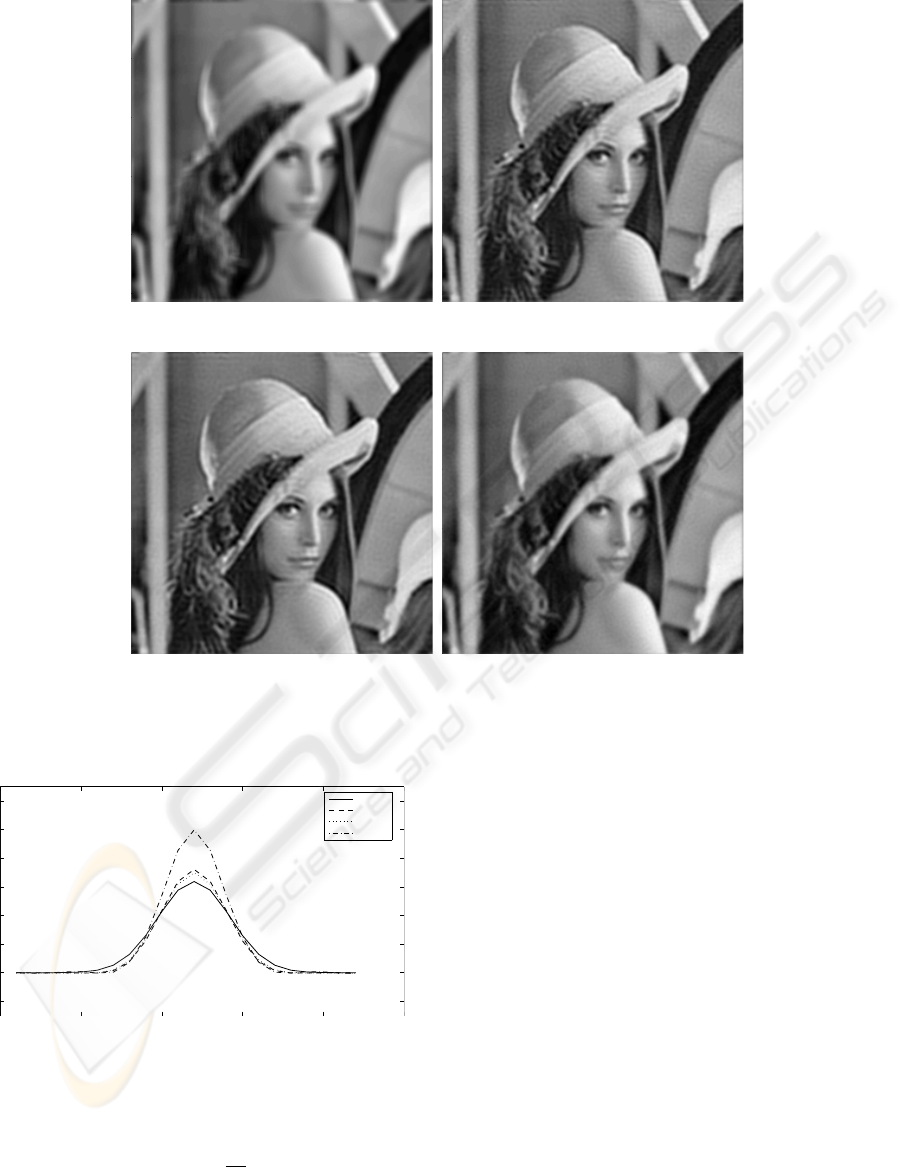
In the first artificial experiment the blurring PSF
was set to a Gaussian function, with variance σ
2
h
= 5.
We initialized all methods, using a Gaussian PSF with
variance σ
2
h
i
n
= 3. The kernel function that was used
by the kernel based methods was again a Gaussian
function with variance σ
2
φ
= 2. The estimated images
of the compared algorithms are shown in fig. 2 and the
estimated PSFs in fig. 3. The corresponding ISNRs
are shown in table 1.
In the next artificial experiment we considered a
7×7 square-shaped PSF. This type of PSF is very dif-
ficult to estimate because of the discontinuities at the
edges of the rectangle. We again initialize the PSF
as a Gaussian shaped function with variance σ
2
h
i
n
= 3.
The kernel function was set to a Gaussian with vari-
ance σ
2
φ
= 1 in order to be flexible enough to model
the boundaries of the square. The estimated images of
the compared algorithms are shown in fig. 4 and the
PSFs in fig. 5. The corresponding ISNRs are shown
in table 1.
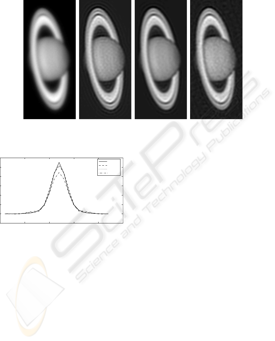
5.2 Experiments on Real Astronomical
Images
We also applied the methodology on a real astronom-
ical image of the Saturn planet, which has previously
been used in (Molina et al., 2006). Previous studies
have suggested the following symmetric approxima-
tion for the PSF of images taken from ground based
ROBUST VARIATIONAL BAYESIAN KERNEL BASED BLIND IMAGE DECONVOLUTION
147

50
100
150
200
250
(a)
50
100
150
200
250
(b)
50
100
150
200
250
(c)
50
100
150
200
250
(d)
Figure 2: Degraded image (a) generated with a Gaussian PSF with σ
2
h
= 5. Estimated image of the (b)RVMBID, (c) rRVMBID
and (d) VAR1 algorithms. The PSF was initialized as a Gaussian with σ
2
hin
= 3 in all cases.
−0.01
0
0.01
0.02
0.03
0.04
0.05
0.06
real
RVMBID
rRVMBID
VAR1
Figure 3: True PSF and PSF estimations for the case of
Gaussian PSF with σ
2
h
= 5.
telescopes:
h(r) ∝ (1+
r
2
R
2
)
−δ
(52)
The parameters δ and R can be estimated (Molina
et al., 2006) and are δ ≈ 3 and R ≈ 3.4. The image
estimations of the RVMBID, rRVMBID and VAR1
algorithms are shown in fig. 6 and the PSFs in fig. 7.
The performance of all the variational algorithms
generally depends on the initialization of the param-
eters. This happens because the variational bound
is a non-convex function and therefore depends on
the initialization a different local maximum may be
achieved. In all the above experiments, we sought the
initialization that gave the best results.
6 CONCLUSIONS
We presented a Bayesian treatment of the BID prob-
lem in which the PSF was modeled as a superposi-
tion of kernel functions. We then applied a sparse
prior distribution on this kernel model in order to esti-
mate the support and shape of the PSF. Furthermore,
we assumed a heavy tailed pdf for the noise in or-
VISAPP 2007 - International Conference on Computer Vision Theory and Applications
148

50
100
150
200
250
(a)
50
100
150
200
250
(b)
50
100
150
200
250
(c)
50
100
150
200
250
(d)
Figure 4: Degraded image (a) generated with a rectangular 7 × 7 square PSF (e). Estimated image of the (b) RVMBID, (c)
rRVMBID and (d) VAR1 algorithms. The PSF was initialized as a Gaussian with σ
2
hin
= 3 in all cases.
−0.01
0
0.01
0.02
0.03
0.04
0.05
0.06
real
RVMBID
rRVMBID
VAR1
Figure 5: True PSF and PSF estimations for the case of
rectangular 7× 7 square PSF.
der to achieve robustness. Because of the complexity
of the model, we used the variational framework to
achieve inference. Several experiments have been car-
ried out, that demonstrate the superior performance
of the method with respect to another variational ap-
proach proposed in (Likas and Galatsanos, 2004).
An improvement to the proposed method would
be to allow many different types of kernels at each
pixel. Thus, one could consider, for example, both
rectangular and Gaussian kernels and the best one de-
pending on the true PSF would be selected automati-
cally. Another interesting enhancement to the method
would be to consider a non-stationary prior model for
the image, which would contain a different γ
i
param-
eter for each pixel. This image prior, would model
better edge and textured area, however, there are sev-
eral computational difficulties to be overcome for its
implementation.
ACKNOWLEDGEMENTS
This research was co-funded by the program
‘Pythagoras II’ of the ‘Operational Program for Edu-
ROBUST VARIATIONAL BAYESIAN KERNEL BASED BLIND IMAGE DECONVOLUTION
149

20
40
60
80
100
120
140
(a)
20
40
60
80
100
120
140
(b)
20
40
60
80
100
120
140
(c)
20
40
60
80
100
120
140
(d)
Figure 6: Degraded image (a). Estimated image the (b) RVMBID, (c) rRVMBID and (d) VAR1 algorithms. The PSF was
initialized as a Gaussian with σ
2
hin
= 3 in all cases.
−0.01
0
0.01
0.02
0.03
0.04
0.05
0.06
real
RVMBID
rRVMBID
VAR1
Figure 7: True PSF and PSF estimations for the real saturn
image.
cation and Initial Vocational Training’ of the Hellenic
Ministry of Education.
REFERENCES
Bishop, C. M. (2006). Pattern Recognition and Machine
Learning. Springer.
D.Kundur and D.Hatzinakos (1996). Blind image deconvo-
lution. IEEE Signal Processing Mag., 13(3):43–64.
Galatsanos, N. P., Mesarovic, V. Z., Molina, R., Katsagge-
los, A. K., and Mateos, J. (2002). Hyperparameter es-
timation in image restoration problems with partially-
known blurs. Optical Eng., 41(8):1845–1854.
Jeffs, B. D. and Christou, J. C. (1998). Blind Bayesian
restoration of adaptive optics telescope images using
generalized Gaussian markov random field models.
In Bonaccini, D. and Tyson, R. K., editors, in Proc.
SPIE. Adaptive Optical System Technologies, volume
3353, pages 1006–1013.
Jordan, M., Gharamani, Z., Jaakkola, T., and Saul, L.
(1998). An introduction to variational methods for
graphical models. In Jordan, M., editor, Learning in
Graphical Models, pages 105–162. Kluwer.
Kundur, D. and Hatzinakos, D. (1996). Blind image de-
convolution revisited. IEEE Signal Processing Mag.,
13(6):61–63.
Likas, A. and Galatsanos, N. P. (2004). A variational ap-
proach for Bayesian blind image deconvolution. IEEE
Trans. on Signal Processing, 52:2222–2233.
Molina, R., Mateos, J., and Katsaggelos, A. (2006). Blind
deconvolution using a variational approach to parame-
ter, image, and blur estimation. IEEE Trans. on Image
Processing, to appear.
Peel, D. and Mclachlan, G. J. (2000). Robust mixture mod-
elling using the t distribution. Statistics and Comput-
ing, 10(4):339–348.
Tipping, M. E. (2001). Sparse Bayesian learning and the
relevance vector machine. Journal of Machine Learn-
ing Research, 1:211–244.
Tipping, M. E. and Lawrence, N. D. (2003). A variational
approach to robust Bayesian interpolation. In IEEE
Workshop on Neural Networks for Signal Processing,
pages 229–238.
Tzikas, D., Likas, A., and Galatsanos, N. (2006a). Large
scale multikernel RVM for object detection. In SETN,
pages 389–399.
Tzikas, D., Likas, A., and Galatsanos, N. (2006b). Varia-
tional Bayesian blind image deconvolution based on a
sparse kernel model for the point spread function. In
in Proc. EUSIPCO.
VISAPP 2007 - International Conference on Computer Vision Theory and Applications
150