USE A NEURAL NETWORKS TO ESTIMATE AND TRACK THE
PN SEQUENCE IN LOWER SNR DS-SS SIGNALS
Tianqi Zhang
1
, Shaosheng Dai
1
1
InstituteSchool of Communication and Information Engineering / Institute of Signal Processing and System On Chip
(ISPSOC), Chongqing University of Posts and Telecommunications (CQUPT), Chongqing 400065, China
Zhengzhong Zhou
2
, Xiaokang Lin
3
2
School of Communication and Information Engineering, University of Electronic Science and Technology of China
(UESTC), Chengdu 610054, China
3
Graduate School at Shenzhen of Tsinghua University, Shenzhen 518055, China
Keywords: Generalized Hebbian algorithm (GHA), neural network (NN), direct sequence spread spectrum (DS-SS)
signals, pseudo noise (PN) sequence.
Abstract: This paper proposes a modified Sanger’s generalized Hebbian algorithm (GHA) neural network (NN)
method to estimate and track the pseudo noise (PN) sequence in lower signal to noise ratios (SNR) direct
sequence spread spectrum (DS-SS) signals. The proposed method is based on eigen-analysis of DS-SS
signals. The received signal is firstly sampled and divided into non-overlapping signal vectors according to
a temporal window, which duration is a periods of PN sequence. Then an autocorrelation matrix is
computed and accumulated by these signal vectors one by one. The PN sequence can be estimated and
tracked by the principal eigenvector of autocorrelation matrix in the end. But the eigen-analysis method
becomes inefficiency when the estimated PN sequence becomes longer or the estimated PN sequence
becomes time varying. In order to overcome these shortcomings, we use a modified Sanger’s GHA NN to
realize the PN sequence estimation and tracking from lower SNR input DS-SS signals adaptively and
effectively.
1 INTRODUCTION
Since the direct sequence spread spectrum (DS-SS,
DS) signals have the distinguished capability of anti-
jamming and lower probability interception, the DS
signals have used broadly in communication, radar,
telemetry and telecommand etc for a long time.
Usually, the spread spectrum receiver has to perform
synchronization before it can start the despreading
operation. For the case of DS, this entails
establishing complete knowledge of the pseudo
noise (PN) sequence and the timing.
Synchronization is performed in two stages. The
first stage of coarse synchronization is known as PN
acquisition and the final stage of maintaining the
fine synchronization is called PN tracking. While
PN tracking forms an important part of DS
synchronization, PN acquisition is a more
challenging problem.
Conventional acquisition techniques (Simnon et
al., 1994) rely on the knowledge of the internal
algebraic structure of the PN spreading sequence to
establish synchronization. While they demonstrate
good acquisition performance in low noise
environments, they tend to break down in
environments with high levels of noise and
interference because of a high false alarm rate.
Furthermore, reliable algebraic techniques for
synchronization have yet to be developed for
nonlinear codes, or codes with unknown code
structure, chip constellations, and residual delay.
Additionally, the PN sequences of DS signal have
the distinguished function of keeping secrecy. If you
have no knowledge of the PN sequence, you could
not demodulate the transmitted message symbols
generally.
A method of autocorrelation and cyclic
autocorrelation was proposed to de-spread the DS
379
Zhang T., Dai S., Zhou Z. and Lin X. (2007).
USE A NEURAL NETWORKS TO ESTIMATE AND TRACK THE PN SEQUENCE IN LOWER SNR DS-SS SIGNALS.
In Proceedings of the Fourth International Conference on Informatics in Control, Automation and Robotics, pages 379-384
DOI: 10.5220/0001647003790384
Copyright
c
 SciTePress

signal (French et al., 1986), which can extract a
differentially-encoded estimate of the underlying
message sequence from a modulation-on-symbol DS
signal (where the spreading PN sequence repeats
once per message symbol) on the basis of the
periodic structure of these signals. This method
attempts to overcome some of these disadvantages
by making no assumptions about the internal
algebraic structure of the PN spreading sequence.
They can operate in the presence of arbitrary delay
and for arbitrary codes or chip constellations.
Because some spectral correlation computations are
required, it is difficult to carry out in real-time.
Furthermore, it does only de-spread the DS signal
without the PN sequence, but it doesn’t utilize or
analyze any signal structure information. So far,
most of DS packet radio and military systems often
require frequent, fast and robust synchronization.
Blind estimation and tracking of the PN spreading
sequence without the a priori knowledge of its
structure and timing is useful in achieving these
objectives.
The signal subspace analysis and relational
techniques, introduced in (Zhang et al., 2005) (Simic
et al., 2005) (Zhan et al., 2005), is precisely such a
technique. It is based on the signal subspace analysis
of DS signal, and estimates the PN spreading
sequence blindly by exploiting cyclostationarity
property and eigenstructure of the DS signal. The
technique provides perfect estimates of the PN
spreading sequence under the assumptions of infinite
time-averaging in the presence of arbitrary levels of
temporally-white background noise. But the
methods proposed in (Zhang et al., 2005) (Simic et
al., 2005) (Zhan et al., 2005) belong to a batch
method, when the number of samples in a period of
observation window becomes too large or the
estimated PN sequence becomes time-varying, the
computation of matrix decomposition may not be
feasible in practice.
This paper proposes an unsupervised adaptive
approach of Sanger’s generalized Hebbian algorithm
(GHA) neural networks (NN) to PN sequence blind
estimation and adaptive tracking. It needs the first
and second principal component vectors associated
with the largest and second largest eigenvalue
respectively; and it can deal with too long sampling
signal vectors and time-varying cases.
2 SIGNAL MODEL
The base band DS signal
()
x
t
corrupted by the white
Gaussian noise
()nt
with the zero mean and
2
n
σ
variance can be expressed as (French et al., 1986)
(Zhang et al., 2005) (Simic et al., 2005) (Zhan et al.,
2005)
() ( ) ()
x
x
tstT nt
=
−+
(1)
Where
() () ()
s
tdtpt
=
is the DS signal ，
() ( )
jc
j
pt pqt jT
∞
=−∞
=−
∑
，
{
}
1
j
p ∈±
is the periodic
PN sequence ，
0
() ( )
k
k
dt mqt kT
∞
=−∞
=−
∑
，
{
}
1
k
m
∈
±
is the symbol bits, uniformly distributed
with
[]()
kl
E
mm k l
δ
=
−
，
()
δ
⋅
is the Dirac function,
()qt
denotes a pulse chip. Where
0 c
TNT=
，
N
is
the length of PN sequence，
0
T
is the period of PN
sequence，
c
T
is the chip duration,
x
T
is the random
time delay and uniformly distributed on the
0
[0, ]T
.
According to the above, the PN sequence and
synchronization are required to de-spread the
received DS signals. But in some cases, we only
have the received DS signals. We must estimate the
signal parameters firstly (We assume that
0
T
and
c
T
had known in this paper), and then estimate the PN
sequence and synchronization.
3 SUBSPACE ANALYSIS BASED
ON K-L TRANSFORMATION
The received DS signal is sampled and divided into
non-overlapping temporal windows, the duration of
which is
0
T
. Then one of the received signal vector
is
() () ()kkk
=
+Xsn
，
",3,2,1=k
(2)
Where
()ks
is the
k
-th vector of useful signal,
(
)
kn
is the additive white Gaussian noise vector. The
dimension of vector
()kX
is
0
/
c
N
TT=
. If the
random time-delay is
x
T
，
0
0 TT
x
<≤
,
() ks
may
contain two consecutive symbol bits, each
modulated by a period of PN sequence, i.e.
112
()
kk
km m
+
=
+spp
(3)
ICINCO 2007 - International Conference on Informatics in Control, Automation and Robotics
380

Where
k
m
and
1+k
m
are the two consecutive symbol
bits,
1
p
(
2
p )
is the right (left) part of the PN
sequence waveform.
According to K-L transformation, we normalize
i
p by
/
iii
=upp
,
1, 2i =
()
T
ij
ij δ =−uu
，
,1,2ij=
(4)
Where
1
u
and
2
u
are ortho-normal vectors,
()
δ
⋅
is a
Dirac function.
From
1
u
and
2
u
, we have
11 1 2 2
() ()
kk
km m k
+
=+ +Xpupun
(5)
The autocorrelation matrix of
()kX
:
X
R
may be
estimated as
()
1
1
ˆ
() ()
M
T
X
i
M
ii
M
=
=
∑
RXX
(6)
Assume
()ks
,
()kn
are mutually independent,
substitute Eq.(5) into Eq.(6) yields
2
0
11 2 2
ˆ
()
TT
XX sssnnn
TT
xx
nSNR SNR
cc
TT T
TT
σγ γ
=∞= +
⎧⎫
⎛⎞⎛⎞
−
⎪⎪
=⋅⋅+⋅⋅+
⎨⎬
⎜⎟⎜⎟
⎪⎪
⎝⎠⎝⎠
⎩⎭
RR UΛ UUΛ U
uu uu I
(7)
Where
I
is an
identity
matrix of dimension
N
N
×
,
the expectation of
k
m
is zero. The variance of
k
m
is
2
m
σ
, the symbol is uncorrelated from each other. The
energy of PN sequence is
2
pc
ET≈ p
，the variance
of
() ks
is
0
22
TE
pms
σσ =
，
22
SNR s n
γ
σσ =
.
The row
vectors of
s
U
and
n
U
are corresponding to the
eigenvectors of eigenvalue
()
2
10
1
R
SNR x c n
TTT
λγ
σ =+ ⋅ −⎡⎤
⎣⎦
,
()
2
2
1
R
SNR x c n
TT
λγ
σ =+ ⋅
and
2
n
σ
, and exist
2
21 nRR
σλλ >≥
. It is clear that the eigenvalues of
X
R
are dependent on
x
T
.
It is shown in (Anderson,
1963) that the estimated principal eigenvectors have
the following behavior:
(
)
log log / , 1, 2, ,
ii
OMMiK−= =uu " .
Therefore,
M →∞, there always exists
ii
=
uu
,
1, 2, ,iK = "
.
When
0≠
x
T
, the biggest eigenvalue is
1R
λ
, the
sign of its corresponding eigenvector
11
sign( )=pu
.
The second biggest eigenvalue is
2R
λ
and the sign of
its corresponding eigenvector
22
sign( )=pu
. We can
recover a period PN sequence from
21 2 1
sign( ) sign( )=+= +pp p u u
. When
0
=
x
T
,
1R
λ
and
11
sign( )=pu
which denote a period of PN
sequence.
Because the accumulation of
X
R
estimation by
Eq.
（6） is a de-noise process, we can estimate the
PN sequence by decomposition of
ˆ
X
R
even when
SNR
γ
is lower. However, the memory size and
computational speed will become problems when
N
becomes bigger. Additionally, it is difficult to use
this batch method to realize the
PN tracking of DS
signals.
Since we would like to track slowly varying
parameters, we must form a moving average
estimate of the correlation matrix based on the
J
most recent observations
()
1
1
ˆ
,()()
i
T
X
jiJ
iJ j j
J
=− +
=
∑
RXX
(8)
It is well known (Anderson, 1963) that the
maximum likelihood estimate of the eigenvalues and
associated eigenvectors of
X
R
is just the eigenvalue
decomposition of
(
)
ˆ
,
X
iJR
. But there are a lot of
difficulties in this tracking process by eigenvalue
decomposition for it’s a batch method. In the
following context, we will propose to use the PCA
NN to solve these problems.
4 IMPLEMENTATION OF A
MODIFIED SANGER’S GHA
NEURAL NETWORKS
According to the result of subspace analysis of DS
signals based on K-L transformation, we’ll have to
extract the first and second principal eigenvectors
before realizing the whole PN sequence estimation.
A two-layer PCA NN is used to estimate the PN
sequence in DS signal blindly as in Fig.1. The
number of input neurons is given by
0 c
NTT=
.
0
x
1
x
2
x
1N
x
−
1
y
2
y
01
w
11
w
21
w
(1)1N
w
−
01
w
11
w
21
w
(1)1N
w
−
0
x
′
1
x
′
2
x
′
1N
x
−
′
02
w
12
w
22
w
(1)2N
w
−
+
+
+
+
−
−
−
−
+
+
+
+
+
+
Figure 1: Neural Networks.
Assume
0
x
T
≠
, one of the received signal vectors
is
USE A NEURAL NETWORKS TO ESTIMATE AND TRACK THE PN SEQUENCE IN LOWER SNR DS-SS SIGNALS
381

[]
[]
01 1
() ( ) (), ( ), , ( 1)
(), (), , ()
T
CC
T
N
t k xt xt T xt N T
xtxt x t
−
⎡⎤
== − −−
⎣⎦
=
XX
"
"
(9)
Where
{
}
() ( ), 0,1, , 1
iC
xt xt iT i N=− = − "
are sampled by
one point per chip. The synaptic weight vector is
01 (1)
() (), (), , ()
T
jjj Nj
twtwt w t
−
⎡⎤
=
⎣⎦
w
"
(10)
Where the sign of {
()
ij
wt
，
0,1, , 1iN=−"
,
1, 2j
=
}
denotes the 1
st
and 2
nd
i-th bit of estimated PN
sequence. The output layer of NN has only two
neurons, its output is
1
0
() () (), 1,2
N
jiji
i
yt wtxt j
−
=
= =
∑
(11)
The synaptic weight
()
ij
wt
is adapted in
accordance with a general form of Hebbian learning,
as shown by
1
(1) () () () ()()
j
jjjj kk
k
ttyttytt β
=
⎡
⎤
+= + −
⎢
⎥
⎣
⎦
∑
ww X w
(12)
Where
j
β
are the positive step-size parameters. In
order to achieve good robust convergence
performance, we modified
j
β
in learning rule
Eq.(12) of Sanger’s GHA as follows
1/ ( 1),
jj
dt
β
=+
2
(1) () (), 1,2
jjjj
dt Bdt yt j+= + =
(13)
Where
,1,2
j
Bj =
, are two positive constants
(usually less than 1). Where the Sanger’s
generalized Hebbian algorithm (GHA) of Eq.(12) for
layer of
j
neurons includes the algorithm of original
Hebbian for a single neuron as a special case ,that is,
1
j
=
.
For a heuristic understanding of how the
Sanger’s GHA actually operates, we use matrix
notation to rewrite the version of the algorithm
defined in Eq.(12) as follows
(1) () () () () ()
jjjj jj
ttyttytt β
′
⎡
⎤
+= + −
⎣
⎦
ww X w
(14)
Where
1
1
() () () ()
j
kk
k
tt ytt
−
=
′
=−
∑
XX w
(15)
The vector
()t
′
X
represents a modified form of
the input vector. Provided that the first neuron has
already converged to the first principal component,
the second neuron sees an input vector
()t
′
X
from
which the first eigenvector of the correlation matrix
X
R
has been removed. The second neuron therefore
extracts the first principal component of
()t
′
X
,
which is equivalent to the second principal
component of the original input vector
()tX
.
The neuron-by-neuron description above is
intended merely to simplify the explanation. In
practice, all the neurons in this modified generalized
Hebbian algorithm tend to converge together. There
is a convergence theorem in (Sanger, 1989) (Haykin,
1999) which can guarantee the convergence of the
modified Sanger’s GHA NN. It guarantees the GHA
NN to find the first
j
eigenvectors of the correlation
matrix
X
R
. Equally important is the fact that we do
not need to compute
X
R
. Rather, the first
j
eigenvectors of
X
R
are computed by the algorithm
directly from the input signal. The resulting
computational savings can be enormous especially if
the dimensionality
N
of the input space is very
large, and the required number of the eigenvectors
associated with the
j
largest eigenvalues of the
X
R
is a small fraction of
N
. This provides best
advantage to track the time-varying PN spreading
sequence of DS signals adaptively.
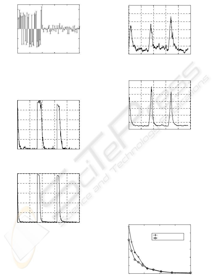
5 SIMULATIONS
The experiments mainly focus on the NN
implementation. We get principal eigenvectors and
performance curves.
0 20 40 60 80 100
-0.2
-0.15
-0.1
-0.05
0
0.05
0.1
0.15
0.2
time
the first principal eigenvector
Tx=40Tc
Figure 2: The estimated 1st principal eigenvector.
ICINCO 2007 - International Conference on Informatics in Control, Automation and Robotics
382

0 20 40 60 80 100
-0.2
-0.1
0
0.1
0.2
time
the second principal eigenvector
Figure 3: The estimated 2nd principal eigenvector.
Fig.2 and Fig.3 denote the first and second principal
eigenvector with N=100bit at Tx=0.4T0. From them,
we may estimate the parameter Tx and reconstruct
the original PN sequence.
0 500 1000 1500 2000 2500
0
0.2
0.4
0.6
0.8
1
data group number
bit error rate
N=100bit
SNR=-12.041dB
Figure 4: Tthe performance curves of PN tracking.
0 500 1000 1500 2000 2500
0
0.2
0.4
0.6
0.8
1
data group number
bit error rate
N=1000bit
SNR=-12.041dB
Figure 5: The performance curves of PN tracking.
0 500 1000 1500 2000 2500
1
1.5
2
2.5
3
3.5
4
x 10
-4
data group number
beta1(t)
N=100bit
SNR=-12.04dB
Figure 6: The curve of
1
()t
β
.
0 500 1000 1500 2000 2500
1
2
3
4
5
6
7
8
x 10
-5
data group number
beta1(t)
N=1000bit
SNR=-12.04dB
Figure 7: the curve of
1
()t
β
.
Fig.4-5 show the tracking performance of the NN
under
SNR=-12.04dB when the length of PN
sequence is
N=100bit and N=1000bit respectively.
Fig.6-7 show the curves of step-size
1
()t
β
when the
case of
N=100bit, SNR=-12.04dB and N=1000bit,
SNR=-12.04dB
, respectively. Under the same
parameters except the length and content of PN
sequence, we study the convergence behavior of the
NN in signal scenarios with sudden PN sequence
changes. We see in Fig.4-7 that when the PN
sequence is longer, the convergence and tracking
performance is better.
-20 -15 -10 -5 0
0
500
1000
1500
2000
2500
3000
SNR(dB)
the average number of data group
N=100bit, Tx=40Tc
N=1000bit,Tx=400Tc
Figure 8: The performance curves of PN estimation.
USE A NEURAL NETWORKS TO ESTIMATE AND TRACK THE PN SEQUENCE IN LOWER SNR DS-SS SIGNALS
383

Fig.8 denotes the performance curves of PN
sequence estimation. It shows the time taken for the
NN to perfectly estimate the PN sequence for
lengths of
N=100bit and N=1000bit at T
x
/T
0
=0.4.
Under the same condition, when the longer the PN
sequence is, the better the performance is.
6 CONCLUSIONS
A modified Sanger’s GHA NN technique for blind
estimation and adaptive tracking of PN sequence of
DS signals is developed and demonstrated. The
technique, referred to here as the modified Sanger’s
GHA NN algorithm, exploits the subspace analysis
based on K-L transformation of the DS signal to
blindly estimate and adaptively track the spreading
code and can further despread the underlying
message sequence, without knowledge of the content
of the PN code or message sequences. The technique
is applicable to arbitrary spreading codes and
message sequences, and can operate in environments
containing arbitrary levels of additive white
Gaussian noise in theory.
The technique is demonstrated for the length of
PN code
N=100bit and 1000bit DS-SS signal
received in
-20 dB to 0 dB of additive white
Gaussian noise. It is shown that the technique can
blindly estimate and adaptively track the PN
sequence in the presence of strong additive white
Gaussian noise. In (Simic et al., 2005) Simic used
the method of eigen-analysis to achieve –5dB of the
SNR threshold, moreover, in (Zhan et al., 2005)
Zhan use the method of matrix to achieve –12dB
SNR
threshold, but we can realize threshold of
dBSNR 0.20−=
easily here, hence the performance
of the methods in this paper is more better. The
convergence time of the algorithm for PN sequence
perfect estimation is also shown to be competitive
with conventional despreading techniques (which
require knowledge of the spreading code) such as
delay-lock loops.
These results show that modified Sanger’s
GHA NN technique can provide a promising
alternative to existing despreading algorithms. The
algorithm can be applicable to signals with short
code lengths, such as commercial communication
signals. The algorithm can be also applicable to
signals with longer code lengths, such as military
communication signals. It can be further used in
management and scout of DS communications.
ACKNOWLEDGEMENTS
This work is supported by the National Natural
Science Foundation of China (No.60602057), the
Natural Science Foundation of Chongqing
University of Posts and Telecommunications
(CQUPT) (No.A2006-04
， No.A2006-86), the
Natural Science Foundation of Chongqing
Municipal Education Commission (No.KJ060509),
and the Natural Science Foundation of Chongqing
Science and Technology Commission (No.
CSTC2006BB2373).
REFERENCES
M. K. Simon, J. K. Omura, R. A. Scholtz, and B. K.
Levitt,
Spread Spectrum Communications Handbook.
New York: McGraw-Hill, 1994.
C. A. French and W. A. Gardner, “Spread spectrum
despreading without the code,” IEEE Trans.
Cornmun.,
vol. COM-34, pp. 404-408, Apr. 1986.
Tianqi Zhang, Xiaokang Lin and Zhengzhong Zhou,
“Blind Estimation of the PN Sequence in Lower SNR
DS/SS Signals ， ”
IEICE Transaction On
Communications
, Vol.E88-B, No.7, JULY, 2005, pp.
3087-3089.
Simic, S. and Zejak, A., “Blind Estimation of the Code
Sequence in Spread Spectrum Radar,”
the 7th
International Conference on Telecommunications in
Modern Satellite, Cable and Broadcasting Services,
IEEE-TELSIKS, 2005
. Vol.2, 28-30 Sept. 2005, pp:
485 – 490.
Zhan, Y., Cao Z., and Lu J., “Spread-spectrum sequence
estimation for DSSS signal in non-cooperative
communication systems,”
IEE Proc.-Commun,
Vol.152, No.4, 2005, pp.476-480.
T.D. Sanger, “Optimal unsupervised learning in a single-
layer linear feedforward neural networks,”
Neural
Networks
, vol.3, pp.459-473, 1989.
S. Haykin,
Neural Networks—A Comprehensive
Foundation
. Prentice Hall PTR, Upper Saddle River,
NJ, USA, 1999.
T.W. Anderson. Asymptotic theory for principal
component analysis.
Ann. Math. Statist., 1963, 35:
1296-1303.
ICINCO 2007 - International Conference on Informatics in Control, Automation and Robotics
384