PRELIMINARY TESTS OF THE REMS GT-SENSOR

Eduardo Sebastián and Javier Gomez-Elvira

Lab. de Robótica y Exploración Planetaria, Centro de Astrobiología, Ctra. Ajalvir Km.4, Torrejón de Ardoz, Spain

Keywords: Environmental monitoring, infrared temperature detector, system identification and sensor calibration.

Abstract: This paper describes and tests a mathematical model of the REMS GT-sensor (Ground Temperature), which

will be part of the payload of the NASA MSL mission to Mars. A short review of the instrument most

critical aspects like the in-flight calibration system and the small size, are presented. It is proposed a

mathematical model of the GT-sensor based on an energy balance theory, which considers the internal

construction of the thermopile, and allows the designer to model independently the change in any of its

parameters. The instrument includes an in-flight calibration system which accounts for dust build up on the

thermopile window during operations. Pre-calibration tests of the system are presented, demonstrating the

good performance of the proposed model, as well as some required improvements.

1 INTRODUCTION

This paper describes a set of preliminary tests to

validate a mathematical model of the REMS (Rover

Environmental Mars Station) GT-sensor (Ground

Temperature). The REMS is a meteorological station

designed at the Centro de Astrobiología, which is

part of the payload of the MSL (Mars Science

Laboratory) NASA mission to Mars. This mission is

expected to be launched in the final months of 2009.

The detection of Mars surface temperature is

essential to develop meteorological models of Mars

atmospheric behavior

(Richardson et al., 2004).

Mars suffers very extreme ground temperature

gradients, from -135ºC to 40ºC between winter and

summer. Also, differences of ±40ºC between the

ground and the atmosphere at 1.5m over the surface

are expected (Smith et al., 2004).

The GT-sensor, as its name indicates, is

dedicated to measure the brightness temperature of

the Mars surface, using an infrared detector that

measures the emitted thermal radiation. The detector

focuses a large surface area, which is far enough

from the rover as to minimize its influence,

measuring the average temperature and avoiding

local effects. The main GT-sensor requirement is to

achieve an accuracy of 5K, in which the errors

created by rover influence, ground emissivity

uncertainty and sensor noise must be included.

The selected infrared detector is a thermopile.

These sensors have the advantage that they can work

at almost any operational temperature, are small and

lightweight and comparative cheap, as well as they

are sensible to all the infrared spectra. Taking into

account the restricted resources available for the

REMS, there is hardly any alternative to

thermopiles. Contrary, thermopiles are not standard

parts for space or military applications. Therefore, at

present no formally space qualified thermopile

sensors exist. It should be noted here, that the IRTM

experiment on the VIKING mission and the MUPUS

experiment of the ROSETA mission have proven the

suitability of this kind of detector to measure low

object temperatures under space conditions.

The paper is organized as follows; section 2

introduces a brief description the REMS GT-sensor.

In section 3 the mathematical model of the sensor is

presented. Section 4 shows preliminary real tests

results, using the proposed model. Finally, section 5

summarizes the results.

2 THE REMS GT-SENSOR

The GT-sensor measures the emitted radiation of the

Mars surface in two infrared wavelength channels,

by using two detectors, looking directly to ground

without any optical system. The selected

measurement channels of the thermopiles are the 8-

14μm and 16-20μm (Vázquez et al., 2005)

. These

channels avoid the abortion band of the CO

centred

in 15μm (Martin, 1986), and minimize the influence

103

Sebastián E. and Gomez-Elvira J. (2007).

PRELIMINARY TESTS OF THE REMS GT-SENSOR.

In Proceedings of the Fourth International Conference on Informatics in Control, Automation and Robotics, pages 103-107

DOI: 10.5220/0001638801030107

 SciTePress

of sun radiation. The thermopiles are of the model

TS-100 (IPHT, 2007), previously used for the

ROSETA mission, which include a RTD sensor and

a filter build to the specification and pre-bonded

onto them as the thermopile window.

The use of two measurement channels is justified

in two ways. First, each channel is specialised in the

measure of a temperature range, based on the Planck

law and higher S/N ratio. And second, the output

signal of the two channels can be combined in order

to apply colour pyrometry techniques. This can help

to estimate the emissivity of the Mars ground,

despite both channels appears to have nearly unit

emissivity (Vázquez et al., 2005).

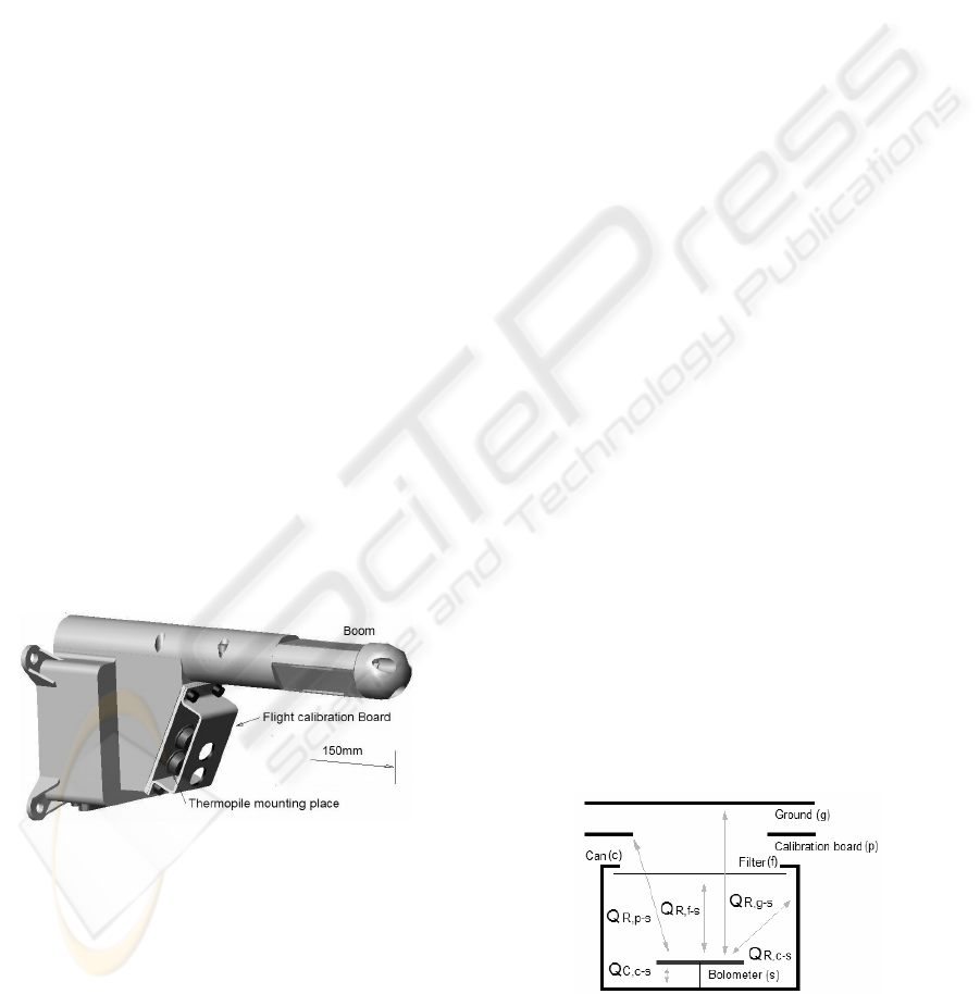
The thermopiles are mounted inside a boom,

figure 1, which is placed in the rover mast at 1.5m

height. The boom has the form of a small arm of

150mm long, and it also hosts the electronics

dedicated to amplify thermopiles signal. The boom

is made of aluminium and is used as a thermal mass

to ensure and acceptably low drift in thermopiles

temperature. The boom’s form permits to avoid the

existence of lateral lobules in the thermopile FOV

(field of view), minimizing the rover direct vision.

The GT-sensor includes an in-flight calibration

system whose main goal is to compensate the

detector degradation due to the deposition of dust

over its window (Richardson et al., 2004). The

system is implemented, without moving parts, by a

high emissivity, low mass calibration plate at a

temperature of our choosing. It is placed in front of

each detector, so that each detector looks at the

ground through a hole in the plate. In this way the

part of the FOV obstructed by the calibration system

is an annulus, limiting the measurement solid angle.

Figure 1: REMS boom and thermopile sensors.

3 MATHEMATICAL MODEL

Usually, the mathematical equation to model a

thermopile considers it as a black box with an input,

the incident energy, and an output, the output

voltage. Therefore, a thermopile is characterised

using a gain with units [V/W], which depends on

thermopile temperature. This equation behaves

properly for high target temperatures, and when no

thermopile worsening is expected during operation.

Essentially, if there is degradation, a parameterized

model is required in order to compensate it.

Contrary, the proposed model is based on an

energy balance theory (Richardson et al., 2004)

which considers the internal thermopile structure

and operation. It behaves better for low target

temperatures, and for a wide range of thermopile

temperatures. It also permits to establish adaptation

algorithms for the change in model parameters.

3.1 Thermopile Model Equations

The proposed model uses two equations. The first

one shows the response of the thermocouples, which

form the thermopile. The thermopile is integrated by

100 thermocouples connected in series and

embedded between the can and the bolometer

(IPHT, 2007). The equation (1) determines the

relation between the thermopile output voltage and

the temperature difference between the hot

(bolometer, T

) and the cold junction (can, T

Therefore, from the measurement of (T

) and the

output voltage (V

out

), the value of T

can be obtained.

))((

cscout

TTTfV −

, (1)

The function

)(

can be approximated by a

polynomial expression provided by the thermopile

manufacturer, which depends on thermopile or can

temperature (T

The second one is the energy balance equation,

and it accounts for the heat fluxes into the

thermopile bolometer from all the bodies around it.

As the bolometer is designed to be well insulated

from the can and to have low thermal mass, the

equilibrium condition of the equation, is reached

after a setting time of a few milliseconds. The

equation considers a simplified model of energy

exchange by thermal radiation (Q

) and conduction

), see figure 2.

Figure 2: GT-Sensor energy terms.

ICINCO 2007 - International Conference on Informatics in Control, Automation and Robotics

104

From the analysis of the energy terms, and after

the thermal equilibrium is reached, the equation (2)

represents the thermal circuit

,,,,,

++++

−−−−− scCscRsfRspRsgR

QQQQQ

(2)

Based on simplified heat flux models, the

equation (2) can be expressed in the following way,

()

()()

()

TTKEEKEEK

EEKEEK

−+−+−

+−+−−=

···

····10

324

αα

(3)

where

represents the factor of the thermopile FOV

obstructed by the flight calibration board, and K

, K

and K

are constants which modulate the

weight of the different terms. These constants

depend on physical factors of the bodies around like:

emissivity, FOV factors, viewed areas, and in the

case of K

on thermal conductance of the materials.

The energy terms

are calculated integrating the

Planck law (4) for each body temperature (T

∫

⎟

⎠

⎞

⎜

⎝

⎛

−=

1·2)·(

dehcTE

λλλ

(4)

where the subscript x represents the body, g(ground),

p(calibration board), f(filter), c(thermopile can) and

s(bolometer). T(

) is the transmittance of the filter.

And the superscript T, I or O denotes if the energy

flux is calculated in the total spectra, in band or out

of filter band respectively.

3.2 Calibration System Equations

The main origin of thermopile degradation, while

operating on Mars conditions, is dust deposition.

During landed operations dust will collect on the

thermopile’s filter. Dust, which has high emisivity,

will block light both into and out the detector, and it

will equilibrate to the same temperature as the filter

it is now in contact. It can therefore be seen as a

changing the area of the filter into something similar

to the can. In other words, if the factor β represent

the part of the FOV that has not been obstructed by

the dust, the equation (3) can be rewritten,

()

(

)

(

)

() ()

()

TTKEEK

EEKEEK

−+−

+−−+−

+−+−−=

··

·)·1(··

·····1·0

ββ

αβαβ

(5)

The equation (5) includes two simplifications:

The filter temperature is supposed to be equal to the

can temperature, and the factor that weights the filter

influence K

is equal to the ground factor (K

), due

to both shares the same FOV.

Therefore, it is the factor β that must be

determined during operations. This can be done by

varying the temperature of the calibration board if

the ground brightness temperature can be trust to

remain constant while the temperature changed

(Smith et al., 2004). The temperature of the

thermopile, the flight calibration board, and the

output voltage of the thermopile must be collected

before and after the temperature changed. Finally,

using the data collected and the equation (5), the

system of equations (6) can be defined,

[

]

111

···0 dcEbEa

+++=

(6.1)

[

]

222

···0 dcEbEa

+++=

(6.2)

where a, b, c and d are a set of known energy terms.

And, the system can be solved for the factor

(

)

212112

· ccEEbdd

−+−−=

(7)

4 TEST RESULTS

In this section, four preliminary experimental tests

dedicated to validate and show the performance of

the sensor model are presented. The tests pretend to

be a simple exercise in ambient conditions of the

experiments to calibrate the REMS GT-sensor.

Prior to start with the description of the tests, it is

necessary to define the experiment setup, figure 3. A

thermopile with a band past filter of 8-14μm,

looking at the calibrated blackbody source

MIKRON M315 and covering its all FOV, was used.

The temperature of the flight calibration board and

the thermopile’s can have been measured using two

individual T type thermocouples, glued to these

elements. The temperatures of both elements have

been controlled using two control systems CAL3200

and the associated thermocouple.

Figure 3: Thermopile model layout and real test model

after dust deposition.

PRELIMINARY TESTS OF THE REMS GT-SENSOR

105

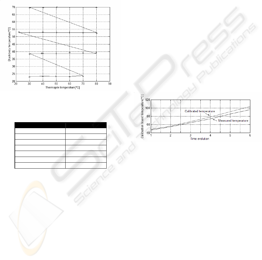
The first test tries to identify the value of those

unknown constants of the thermopile model, table 1.

In order to do it, different blackbody and thermopile

temperatures were consigned, figure 4, while the

flight calibration board was removed, which means

that

is equal to 0. Therefore, based on the energy

balance equation (2), where the energy terms are

known, a least-squares problem for the tested points

is established. Finally, the values of the constants,

which minimize the least-squares error, are obtained.

Figure 4: Real blackbody temperature (-) and estimated

blackbody temperature (*) after the identification process.

Table 1: Thermopile and model variables.

Variable Value

28.1695

128.4088W/K

Error

RMS

0.28K

0.34

Polynomial coefficients [1.0826 -4.0577]

0.415

The second test has been carried out with the

purpose of identifying the factor of the FOV

obstructed by the flight calibration board, this is α.

This value is an essential parameter, necessary for

the flight calibration process.

During the test, the thermopile and the

calibration board must be kept at ambient

temperature, to ensure that their temperatures are

homogeneous and stable. This requirement is

necessary due to the radiance of the flight calibration

has not previously calibrated, and in this way the

error introduced by this factor is avoided. The

blackbody temperature is set over the ambient

temperature. In order to avoid the thermopile

heating, due to the energy radiated by the blackbody,

an opaque surface was introduced in between. This

surface was removed during the measurement time

of bodies temperature and thermopile output. From

these data, the energy terms of equation (2) were

calculated, and we were able to solve for the values

of α, for each blackbody temperature. Finally, these

values of α were averaged in order to obtain a

unique value, table 1.

The third test pretends to know the real

temperature of the calibration board, which is

required to calculate its real radiometric emission.

The test consists of varying the flight calibration

board temperature over the temperature of the

thermopile, while the temperature of the thermopile

and the blackbody are kept constant.

In this case, for each calibration board

temperature, the blackbody and the thermopile

temperatures were collected, as well as the

thermopile’s output. Therefore, based on these data

and the energy valance equation (2), the radiometric

emissions of the flight calibration board are derived,

and from them the real temperatures, which were

compared with the measured temperatures to

determine the absolute calibration error, figure 5.

Also, a first order polynomial, interpolating this

error, has been obtained, table 1.

Figure 5: Temperature calibration error of the flight

calibration board.

The final test is dedicated to analyse the

behaviour of the in-flight calibration algorithm, after

depositing a certain among of dust over the

thermopile window, simulating Mars environment.

The test is divided in two different steps. In the

first one, the flight calibration algorithm is run for

different calibration board temperatures. The figure

6(Top) shows the obtained values of β, with and

without considering the previous calibration of the

calibration board. The data after calibration are more

stable, validating this calibration and reducing

algorithm error. As a result the average value of β is

shown, table 1.

The second step is dedicated to measure the

temperature of the blackbody from: the thermopile

output, the calibrated thermopile model, the

calculated value of the factor β due to dust

deposition. During the test, the temperature of the

blackbody was almost constant, while the

ICINCO 2007 - International Conference on Informatics in Control, Automation and Robotics

106

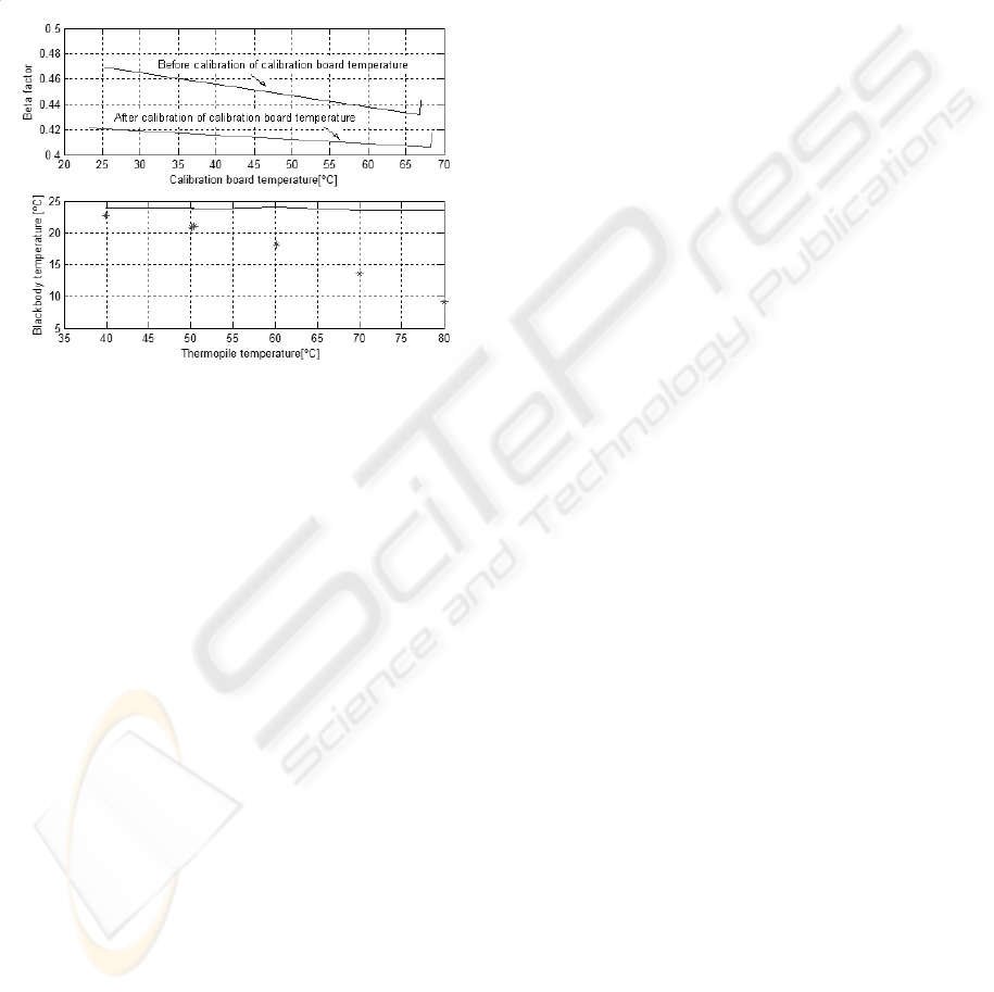
temperature of the thermopile was changed. Figure

6(bottom) shows the result after applying the

measurement algorithm (5) and solving for T

. The

high temperature error is due to the flight calibration

system is calibrating a small surface or annulus in

the external part of the thermopile filter, while the

filter surface used to measure the ground brightness

temperature is in the middle, and the deposition

appears to be no homogeneous. Thus, the

obstruction factor β is higher than the real one.

Figure 6: (top)Value of β factor. (bottom)Real blackbody

temperature (-), and measured blackbody temperature (*).

5 CONCLUSIONS

The thermopile mathematical model presented in

this paper is a valid and precise method to

characterize a thermopile, due to the low least-

squares error of 0.28K for an extensive thermopile

temperature range of almost 60K.

The FOV obstruction factor, generated by the

flight calibration board, reaches a value of 34%. It

can be reduced in order to increase the S/N ratio for

ground temperature signals.

The radiometric calibration of the flight

calibration board is necessary due to the error

introduced by different factors: the calibration of the

temperature sensor, the temperature homogeneity of

the calibration board and the position and anchoring

of the temperature sensor.

Dust deposition, based on dust electrical

characteristics, tends to form small balls around the

union between the thermopile can and window. This

is exactly the area calibrated by the flight calibration

board, justifying the higher value of β. As a future

work, a new calibration system, using a heated

cable, will be studied. The cable will cross the FOV

of the thermopiles, obstructing a homogenous part of

the FOV, and not only a ring in the most external

part. This will minimize the error generated by the

way dust is built up on the window.

ACKNOWLEDGEMENTS

The authors would like to express special thanks to

all members of the REMS project who in different

ways are collaborating in the development of REMS

GT-sensor.

REFERENCES

Richardson M., McEwan I., Schofield T., Smith M.

Souères P., Courdesses M. and Fleury S. 2004.

MIDAS Mars Ice Dust Atmospheric Sounder. MSL

proposal.

Vázquez L., Zorzano M.P., Fernández D., McEwan I.

2005. Considerations about the IR Ground

Temperature Sensor. CAB, REMS Technical Note 1-

101722005. Madrid.

Smith M.D. et al., 2004. First Atmospheric Science

Results from the Mars Exploration Rovers Mini.-TES.

SCIENCE EEE, 306, 1750-1753.

Martin T.Z. 1986. Thermal infrared Opacity Of The Mars

Atmosphere. Icarus, 66, 2-21.

www.ipht-jena.de. 2007. IPHT web page.

PRELIMINARY TESTS OF THE REMS GT-SENSOR

107