INTERCEPTION AND COOPERATIVE RENDEZVOUS BETWEEN
AUTONOMOUS VEHICLES
Yechiel J. Crispin and Marie-Emmanuelle Ricour
Department of Aerospace Engineering, Embry-Riddle Aeronautical University, Daytona Beach, Florida 32114, USA
Keywords:
Multiple Vehicles, Cooperative Rendezvous, Interception, Autonomous Vehicles, Optimal Control, Genetic
Algorithms.
Abstract:
The rendezvous problem between autonomous vehicles is formulated as an optimal cooperative control prob-
lem with terminal constraints. A major approach to the solution of optimal control problems is to seek solutions
which satisfy the first order necessary conditions for an optimum. Such an approach is based on a Hamiltonian
formulation, which leads to a difficult two-point boundary-value problem. In this paper, a different approach is
used in which the control history is found directly by a genetic algorithm search method. The main advantage
of the method is that it does not require the development of a Hamiltonian formulation and consequently, it
eliminates the need to deal with an adjoint problem. This method has been applied to the solution of intercep-
tion and rendezvous problems in an underwater environment, where the direction of the thrust vector is used as
the control. The method is first tested on an interception chaser-target problem where the passive target vehicle
moves along a straight line at constant speed. We then treat a cooperative rendezvous problem between two
active autonomous vehicles. The effects of gravity, thrust and viscous drag are considered and the rendezvous
location is treated as a terminal constraint.
1 INTRODUCTION
In an active-passive rendezvous problem between two
vehicles, the passive or target vehicle does not apply
any control maneuvers along its trajectory. The ac-
tive or chaser vehicle is controlled or guided such as
to meet the passive vehicle at a later time, matching
both the location and the velocity of the target vehi-
cle. In a cooperative rendezvous problem, the two
vehicles are active and maneuver such as to meet at a
later time, at the same location with the same velocity.
The rendezvous problem consists of finding the con-
trol sequences or the guidance laws that are required
in order to bring the two vehicles to a final state of
rendezvous.
An optimal control problem consists of finding the
control histories (control as a function of time) and
the state variables of the dynamical system such as to
minimize a performance index. The differential equa-
tions of motion of the vehicles are then treated as dy-
namical constraints. A possible approach to the so-
lution of the rendezvous problem is to formulate it as
an optimal control problem in which it is required to
find the controls such as to minimize the differences
between the final locations and final velocities of the
vehicles. The methods of approach for solving op-
timal control problems include the classical indirect
methods and the more recent direct methods. The
indirect methods are based on the calculus of varia-
tions and its extension to the maximum principle of
Pontryagin, which is based on a Hamiltonian formu-
lation. These methods use necessary first order con-
ditions for an optimum, they introduce adjoint vari-
ables and require the solution of a two-point bound-
ary value problem (TPBVP) for the state and adjoint
variables. Usually, the state variables are subjected
to initial conditions and the adjoint variables to ter-
minal or final conditions. Two-point boundary value
problems (TPBVP) are much more difficult to solve
than initial value problems (IVP). For this reason, di-
rect methods of solution have been developed which
avoid completely the Hamiltonian formulation. For
149
J. Crispin Y. and Ricour M. (2007).
INTERCEPTION AND COOPERATIVE RENDEZVOUS BETWEEN AUTONOMOUS VEHICLES.
In Proceedings of the Fourth International Conference on Informatics in Control, Automation and Robotics, pages 149-154
DOI: 10.5220/0001631601490154
Copyright
c
 SciTePress

example, a possible approach is to reformulate the
optimal control problem as a nonlinear programming
(NLP) problem by direct transcription of the dynami-
cal equations at prescribed discrete points or colloca-
tion points. This method was originally developed by
Dickmanns and Well (Dickmanns, 1975.) and used by
Hargraves and Paris (Hargraves, 1987) to solve sev-
eral atmospheric trajectory optimization problems.
Another class of direct methods is based on bi-
ologically inspired methods of optimization. These
include evolutionary methods such as genetic algo-
rithms, particle swarm optimization methods and ant
colony optimization algorithms. PSO) mimics the so-
cial behavior of a swarm of insects, see for example
(Venter, 2002), (Crispin,2005). Genetic Algorithms
(GAs) (Goldberg, 1989) are a powerful alternative
method for solving optimal control problems, see also
(Crispin, 2006 and 2007). GAs use a stochastic search
method and are robust when compared to gradient
methods. They are based on a directed random search
which can explore a large region of the design space
without conducting an exhaustive search. This in-
creases the probability of finding a global optimum
solution to the problem. They can handle continuous
or discontinuous variables since they use binary cod-
ing. They require only values of the objective func-
tion but no values of the derivatives. However, GAs
do not guarantee convergence to the global optimum.
If the algorithm converges too fast, the probability of
exploring some regions of the design space will de-
crease. Methods have been developed for preventing
the algorithm from converging to a local optimum.
These include fitness scaling, increased probability of
mutation, redefinition of the fitness function and other
methods that can help maintain the diversity of the
population during the genetic search.
2 COOPERATIVE RENDEZVOUS
AS AN OPTIMAL CONTROL
PROBLEM
We study trajectories of vehicles moving in an incom-
pressible viscous fluid in a 2-dimensional domain.
The motion is described in a cartesian system of co-
ordinates (x,y), where x is positive to the right and
y is positive downwards in the direction of gravity.
The vehicle weight acts downward, in the positive y
direction. The vehicle has a propulsion system that
delivers a thrust of constant magnitude. The thrust is
always tangent to the trajectory. The vehicle is con-
trolled by varying the thrust direction. Since the fluid
is viscous, a drag force acts on the vehicle, in the op-
posite direction of the velocity. The control variable
of the problem is the thrust direction γ(t). The angle
γ(t) is measured positive clockwise from the horizon-
tal direction (positive x direction).
The rendezvous problem is formulated as an opti-
mal control problem, in which it is required to deter-
mine the control functions, or control histories γ
1
(t)
and γ
2
(t) of the two vehicles, such that they will meet
at a prescribed location at the final time t
f
. Since GAs
deal with discrete variables, we discretize the values
of γ(t). We assume that the mass of the vehicles is
constant. The motion of the vehicle is governed by
Newton’s second law and the kinematic relations be-
tween velocity and distance:
d(mV)/dt = mg+ T + D (2.1)
dx/dt = V cosγ (2.2)
dy/dt = V sinγ (2.3)
where D is the drag force acting on the body, V is
the velocity vector, T is the thrust vector and g is the
acceleration of gravity. Since we assumed m is con-
stant,
dV/dt = g+ T/m+ D/m (2.4)
Writing this equation for the components of the
forces along the tangent to the vehicle’s path, we get:
dV/dt = gsinγ + T/m−D/m (2.5)
The drag D is given by:
D =
1
2
ρV
2
SC
D
(2.6)
where ρ is the fluid density, S a typical cross-
section area of the vehicle andC
D
the drag coefficient,
which depends on the Reynolds number Re = ρVd/µ,
where d is a typical dimension of the vehicle and µ
the fluid viscosity.
Substituting the drag from Eq.(2.6) and writing
T = amg, where ais the thrust to weight ratio T/mg,
Eq.(2.5) becomes:
dV/dt = gsinγ + ag−ρV
2
SC
D
/2m (2.7)
Introducing a characteristic length L
c
, time t
c
and
speed v
c
as
L
c
= 2m/ρSC
D
, t
c
=
p
L
c
/g, v
c
=
p
gL
c
(2.8)
the following nondimensional variables can be de-
fined:
ICINCO 2007 - International Conference on Informatics in Control, Automation and Robotics
150

x = L
c
x, y = L
c
y
t = (L
c
/g)
1/2
t, V = (gL
c
)
1/2
V (2.9)
Substituting in Eq.(2.7), we have:
d
V/dt = a+ sinγ(t) −V
2
(2.10)
Similarly, the other equations of motion can be
written in nondimensional form as
d
x/dt = V cosγ(t) (2.11)
dy/dt = V sinγ(t) (2.12)
For each vehicle the initial conditions are:
V(0) = V
0
, x(0) = x
0
, y(0) = y
0
(2.13)
In rendezvous problems, terminal constraints on
the final location can also be required
x(t
f
) = x
f
= x
f
/L
c
y(t
f
) = y
f
= y
f
/L
c
(2.14)
where the nondimensional final time is given by
t
f
= t
f
/
p
L
c
/g
We now define a rendezvous problem between two
vehicles. We denote the variables of the first vehicle
by a subscript 1 and those of the second vehicle by
a subscript 2. We will now drop the bar notation in-
dicating nondimensional variables. The two vehicles
might have different thrust to weight ratios, which are
denoted by a
1
and a
2
, respectively. The equations of
motion for the system of two vehicles are:
dV
1
/dt = a
1
+ sinγ
1
(t) −V
2
1
(2.15)
dx
1
/dt = V
1
cosγ
1
(t) (2.16)
dy
1
/dt = V
1
sinγ
1
(t) (2.17)
dV
2
/dt = a
2
+ sinγ
2
(t) −V
2
2
(2.18)
dx
2
/dt = V
2
cosγ
2
(t) (2.19)
dy
2
/dt = V
2
sinγ
2
(t) (2.20)
The vehicles can start the motion from different
locations and at different speeds. The initial condi-
tions are given by:
V
1
(0) = V
10
, x
1
(0) = x
10
, y
1
(0) = y
10
(2.21)
V
2
(0) = V
20
, x
2
(0) = x
20
, y
2
(0) = y
20
(2.22)
The cooperative rendezvous problem consists of
finding the control functionsγ
1
(t)and γ
2
(t) such as
the two vehicles arrive at a given terminal location
(x
f
,y
f
) and at the same speed in the given time t
f
.The
terminal constraints are then given by:
x
1
(t
f
) = x
f
, x
2
(t
f
) = x
f
y
1
(t
f
) = y
f
, y
2
(t
f
) = y
f
(2.23)
V
1
(t
f
) = V
2
(t
f
)
We can also define an interception problem, of the
target-chaser type, in which one vehicle is passive and
the chaser vehicle maneuvers such as to match the lo-
cation of the target vehicle, but not its velocity. Con-
sistent with the above terminal constraints, we define
the following objective function for the optimal con-
trol problem:
f(x
j
(t
f
),V
j
(t
f
)) =
N
v
∑
j=1



x
j
(t
f
)−x
f



2
+∆V
2
j
(t
f
) = min
(2.24)
where N
v
is the number of vehicles, x
f
= (x
f
,y
f
)
is the prescribed interception or rendezvous point and
∆V
2
j
(t
f
) is the square of the difference between the
magnitudes of the velocities of the vehicles. If we
define the norm as a Euclidean distance, we can write
the following objective function for the case of two
vehicles:
f[x
1
(t
f
), x
2
(t
f
), y
1
(t
f
), y
2
(t
f
), V
1
(t
f
), V
2
(t
f
)] =
= (x
1
(t
f
) −x
f
)
2
+ (x
2
(t
f
) −x
f
)
2
+ (y
1
(t
f
) −y
f
)
2
+(y
2
(t
f
) −y
f
)
2
+ (V
1
(t
f
) −V
2
(t
f
))
2
= min (2.25)
We use standard numerical methods for integrat-
ing the differential equations. The time interval t
f
is divided into N time stepsof duration ∆t = t
f
/N.
The discrete time is t
i
= i∆t.We used a second-order
Runge-Kutta method with fixed time step. We also
tried a fourth-order Runge-Kutta method and a vari-
able time step and found that the results were not sen-
sitive to the method of integration. The control func-
tion γ(t) is discretized to γ(i) = γ(t
i
) according to the
INTERCEPTION AND COOPERATIVE RENDEZVOUS BETWEEN AUTONOMOUS VEHICLES
151

number of time steps N used for the numerical integra-
tion. Depending on the accuracy of the desired solu-
tion, we can choose the number of bits n
i
for encoding
the value of the control γ(i) at each time step i. The
size n
i
used for encoding γ(i) and the number of time
steps N will have an influence on the computational
time. Therefore n
i
and N must be chosen carefully, in
order to obtain an accurate enough solution in a rea-
sonable time. The total length of the chromosome is
given by:
L
ch
= n
i
NN
v
(2.26)
For this problem, we were able to increase the
rate of convergence of the algorithm by introducing
heuristic arguments. For instance, having noticed that
γ(t) is a monotonically decreasing function of time,
we were able to speed up the algorithm by choosing a
function with such a property, a priori. Therefore, in-
stead of waiting for the algorithm to converge towards
a monotonous γ(t), we can sort the values of γ of each
individual solution in decreasing order, before calcu-
lating its fitness. We also use smoothing of the control
function by fitting a third or fourth-order polynomial
to the discrete values of γ. The values of the polyno-
mial at the N discrete time points are then used as the
current values of γ and are used in the integration of
the differential equations.
An appropriate range for γ is γ ∈ [0, π/2]. We
choose N = 30 as a reasonable number of time steps.
We now need to choose the parameters associated
with the Genetic Algorithm. First, we select the
lengths of the “genes” for encoding the discrete val-
ues of γ. A choice of n
i
= 8bits for ∀i ∈[0,N −1] was
made. The interval between two consecutive possible
values of γ is given by:
∆γ = (γ
max
−γ
min
)/(2
n
−1) ≈ 0.0062rad = 0.35deg
For two vehicles and 30 time steps, the length of a
chromosome is then given by:
L
ch
= n
i
NN
v
= 480bits
A reasonable size for the population of solutions is
typically in the range n
pop
∈ [50, 200]. For this prob-
lem, there is no need for a particularly large popula-
tion, so we select n
pop
= 50. The probability of muta-
tion is set to a value of 5 percent p
mut
= 0.05.
3 CHASER-TARGET
INTERCEPTION
We study a chaser-target interception problem be-
tween two vehicles. In this case the first vehicle is
active and the second is passive and moves along
a straight line at a constant depth y
2
= y
f
, constant
speed V
2
and constant angle γ
2
= 0. The two vehicles
start from different points and the interception occurs
at the known depth of the target vehicle y
2
= y
f
. The
horizontal distance x
f
to the interception point is free.
We present the case where the target moves at mod-
erate speed and can be captured by the active chaser
vehicle. Since this is an interception problem, we do
not require matching between the final velocities.
a
1
= a = 0.05, a
2
= 5a = 0.25
t
0
= 0, t
f
= 5
γ
1
∈ [0, π/2] , γ
2
= 0, y
f
= 2 (3.1)
The initial conditions are:
x
1
(0) = x
2
(0) = 0, y
1
(0) = 0
y
2
(0) = y
f
= 2, V
1
(0) = 0
V
2
(0) = V
2
=
p
a
2
+ sinγ
2
=
√
a
2
= 0.5 (3.2)
In order to match the final locations, the following
objective or fitness function is defined:
f[x
1
(t
f
), x
2
(t
f
), y
1
(t
f
)] =
= (x
1
(t
f
) −x
2
(t
f
))
2
+ (y
1
(t
f
) −y
f
)
2
= min (3.3)
The parameters for this test case are summarized
in the following table and the results are given in Figs.
1-3.
N
v
n
pop
n
i
N
2 50 8 30
p
mut
N
gen
γ
1min
γ
1max
0.05 50 0 π/2
a t
0
t
f
(x
01
,y
01
)
0.05 0 5 (0,0)
(x
02
,y
02
) (V
01
,V
02
) x
f
y
f
(0,2) (0,
√
5a) free 2
4 RENDEZVOUS BETWEEN TWO
ACTIVE VEHICLES
We next treat a rendezvous between two vehicles.
The two vehicles start from different points and ren-
dezvous at point (x
f
,y
f
) in a given time t
f
. The vehi-
cles have the same thrust to weight ratio a
1
= a
2
= a.
ICINCO 2007 - International Conference on Informatics in Control, Automation and Robotics
152

0 1 2 3 4 5
0
10
20
30
40
50
60
70
80
90
t
gama (deg))
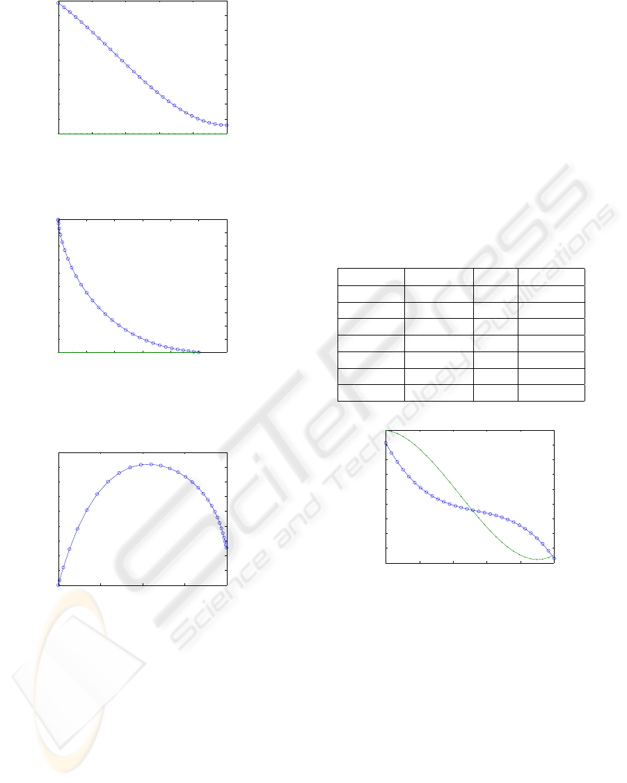
Figure 1: Control function γ
1
(t) and γ
2
= 0 for a chaser-
target interception with prescribed target depth.
0 0.5 1 1.5 2 2.5 3
−2
−1.8
−1.6
−1.4
−1.2
−1
−0.8
−0.6
−0.4
−0.2
0
x / Lc
y / Lc
Figure 2: Trajectories for a chaser-target interception with
prescribed target depth. The sign of y was reversed for plot-
ting.
0 0.5 1 1.5 2
0
0.05
0.1
0.15
0.2
0.25
0.3
0.35
0.4
0.45
v
2
/ 2 g L
c
y / L
c
Figure 3: Kinetic energy as a function of depth for a chaser-
target interception with prescribed target depth.
a
1
= a = 0.05, a
2
= a = 0.05
t
0
= 0, t
f
= 5, x
f
= 2.8, y
f
= 2
γ
1
∈ [0, π/2] γ
2
∈ [0, π/2] (4.1)
with initial conditions:
x
1
(0) = 0, y
1
(0) = 0, x
2
(0) = 0.5, y
2
(0) = 0
V
1
(0) = 0, V
2
(0) = 0 (4.2)
In a rendezvous problem, the objective or fitness
function is given by:
f[x
1
(t
f
), x
2
(t
f
), y
1
(t
f
), y
2
(t
f
), V
1
(t
f
), V
2
(t
f
)] =
= (x
1
(t
f
) −x
f
)
2
+ (y
1
(t
f
) −y
f
)
2
+ (x
2
(t
f
) −x
f
)
2
+(y
2
(t
f
) −y
f
)
2
+ (V
1
(t
f
) −V
2
(t
f
))
2
= min (4.3)
The parameters for this test case are summarized
in the following tableand the results are presented in
Figs.4-5.
N
v
n
pop
n
i
N
2 50 8 30
p
mut
N
gen
γ
1min
γ
1max
0.05 200 0 π/2
a t
0
t
f
(x
01
,y
01
)
0.05 0 5 (0,0)
(x
02
,y
02
) (V
01
,V
02
) x
f
y
f
(0.5,0) (0,0) 2.8 2
0 1 2 3 4 5
0
10
20
30
40
50
60
70
80
90
t
gama (deg))
Figure 4: Control functions γ
1
(t) and γ
2
(t) for rendezvous
between two vehicles with prescribed terminal point.
5 CONCLUSION
The rendezvous problem between two active au-
tonomous vehicles moving in an underwater environ-
ment has been treated using an optimal control for-
mulation with terminal constraints. The two vehicles
have fixed thrust propulsion system and use the direc-
tion of the velocity vector for steering and control. We
use a genetic algorithm to determine directly the con-
trol histories of both vehicles by evolving populations
of possible solutions. An interception problem, where
one vehicle moves along a straight line with constant
INTERCEPTION AND COOPERATIVE RENDEZVOUS BETWEEN AUTONOMOUS VEHICLES
153

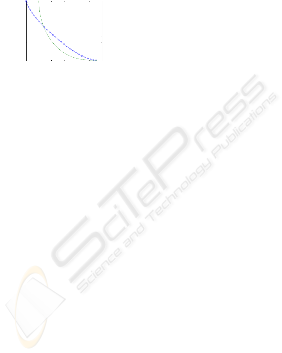
0 0.5 1 1.5 2 2.5 3
−2
−1.8
−1.6
−1.4
−1.2
−1
−0.8
−0.6
−0.4
−0.2
0
x / Lc
y / Lc
Figure 5: Trajectories for rendezvous between two vehicles
with prescribed terminal point.
velocity and the second vehicle acts as a chaser, ma-
neuvering such as to capture the target in a given time,
has also been treated as a test problem. It was found
that the chaser can capture the target within the pre-
scribed time as long as the target speed is below a crit-
ical speed. We then treated the rendezvous problem
between two active vehicles where both the final po-
sitions and velocities are matched. As the initial hori-
zontal distance between the two vehicles is increased,
it becomes more difficult to solve the problem and the
genetic algorithm requires more generations to con-
verge to a near optimal solution.
REFERENCES
Bryson, A. E., “Dynamic Optimization”, 1999, Addison
Wesley Longman.
Crispin, Y., 2005, “Cooperative control of a robot swarm
with network communication delay”, First Interna-
tional Workshop on Multi-Agent Robotic Systems
(MARS 2005), INSTICC Press, Portugal.
Crispin, Y., 2006, “An evolutionary approach to nonlin-
ear discrete-time optimal control with terminal con-
straints”, in Informatics in Control, Automation and
Robotics I, pp.89-97, Springer, Dordrecht, Nether-
lands.
Crispin, Y., 2007, “Evolutionary computation for discrete
and continuous time optimal control problems”, in
Informatics in Control, Automation and Robotics II,
Springer, Dordrecht, Netherlands.
Dickmanns, E. D. and Well, H., 1975, “Approximate so-
lution of optimal control problems using third-order
hermite polynomial functions,” Proceedings of the 6th
Technical Conference on Optimization Techniques,
Springer-Verlag, New York
Goldberg, D.E., 1989, “Genetic Algorithms in Search, Op-
timization and Machine Learning”, Addison-Wesley.
Hargraves, C. R. and Paris, S. W., 1987, “Direct Trajec-
tory Optimization Using Nonlinear Programming and
Collocation”, AIAA Journal of Guidance, Control and
Dynamics, Vol. 10, pp. 338-342
Venter, G. and Sobieszczanski-Sobieski, J.,
2002, “Particle Swarm Optimization”, 43rd
AIAA/ASME/ASCE/AHS/ASC Structures, Struc-
tural Dynamics and Materials Conference.
ICINCO 2007 - International Conference on Informatics in Control, Automation and Robotics
154