HOMOGRAPHY-BASED MOBILE ROBOT MODELING
FOR DIGITAL CONTROL IMPLEMENTATION
Andrea Usai and Paolo Di Giamberardino
Department of Computer and System Sciences “Antonio Ruberti”
University of Rome “La Sapienza”
via Eudossiana 18, Rome, Italy
Keywords:
Nonholonomic mobile robot, multirate digital control, visual servoing.
Abstract:
The paper addresses the development of a kinematic model for a system composed by a nonholonomic mo-
bile robot and a camera used as feedback sensor to close the control loop. It is shown that the proposed
homography-based model takes a particular form that brings to a finite sampled equivalent model. The de-
sign of a multirate digital control is then descibed and discussed, showing that exact solutions are obtained.
Simulation results are also reported to put in evidence the effectiveness of the proposed approach.
1 INTRODUCTION
In several applications a digital implementation of a
controller is required even if the plant dynamics is a
continuous time one.
The classical approach, especially for nonlinear
systems, makes use of a preliminary design of a con-
tinuous time control law that is then implemented in
a digital way by means of a digital device (computer
or microcontroller, for example). In this approach the
digital control law is computed as an approximation
of the continuous time one. This kind of approach is
usually denoted as indirect digital control.
Such an approach can lead to poor controller
performance due to the system approximation per-
formed: the choice of the sampling time affects
the capacity of the digital controller, that generate a
piecewise constant signal, to have a behavior close
enough to the nominal continuous time controller that
assures the desired performances with a continuous
time output signal.
All the works done in the field of visual servoing,
deal with continuous time systems (see, for exam-
ple, in the case of mobile robots: (Chen et al., 2006;
Lopez-Nicolas et al., 2006; Mariottini et al., 2006)).
Image acquisition, elaboration and the nonlinear con-
trol law computation are very time consuming tasks.
So it is not uncommon that the system is controlled, in
a indirect digital control context, with a sampling rate
of 0.5Hz. Clearly this kind of choices strongly affects
the system performances, since the use of a slow rate
in the controller implies that only a slow evolution of
the control system can be required to assure satisfac-
tory behaviors.
To face the drawbacks of poor system approxima-
tion, the trivial solution is slowing down the system
dynamics slowing down the controls variation rate.
This is not always possible, but when the kinematic
model is considered, the system dynamics depends
only on the velocity imposed by the controller (there
is no drift in the model) and so it is quite easy to limit
the effect of a poor system approximation.
In general, taking into account, also in the design
phase, the discrete time nature of the control system
can lead to better closed loop system performances.
This means that the control law designed directly in
the discrete time domain can better address the dis-
crete time evolution of the controlled system. This is
well understood in the linear case and it is also true
for a quite large class of nonlinear systems, the ones
that admits a finite or an exact sampled representation
(Monaco and Normand-Cyrot, 2001). In fact, a neces-
sary step in the design of a digital controller is to deal
with a discrete time plant; if the plant is described by
means of a continuus time dynamics, a discretization
of the plant is required. The possibility of an exact
discretization, better if finite, of the continuous time
model clearly affects the overall performances of the
259
Usai A. and Di Giamberardino P. (2007).
HOMOGRAPHY-BASED MOBILE ROBOT MODELING FOR DIGITAL CONTROL IMPLEMENTATION.
In Proceedings of the Fourth International Conference on Informatics in Control, Automation and Robotics, pages 259-264
DOI: 10.5220/0001631502590264
Copyright
c
 SciTePress

control system since in this case no approximations
are performed in the conversion from continuous time
to discrete time.
2 THE CAMERA-CYCLE MODEL
In this section the kinematic model of the system
composed of a mobile robot (an unicycle) and a cam-
era, used as a feedback sensor to close the control
loop, is presented.
To derive the mobile robot state, the relationship
involving the image space projections of points that
lie on the floor plane, taken from two different camera
poses, are used. Such a relationship is called homog-
raphy. A complete presentation of such projective re-
lations and their properties is shown in (R. Hartley,
2003).
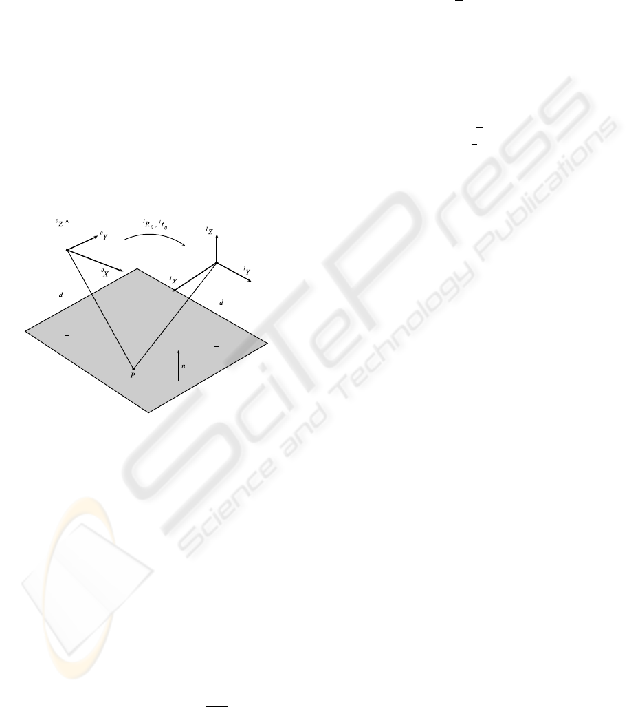
Figure 1: 2-view geometry induced by the mobile robot.
2.1 The Geometric Model
With reference to Figure 1, the relationship between
the coordinates of the point P in the two frames is

1
P
1

=

1
R
0
1
t
0
0 1

0
P
1

(1)
It is an affine relation that becomes a linear one in
the homogeneous coordinate system. If the point P
belongs to a plane in the 3D space with normal versor
n and distance from the origin d, it holds that

n
T
d


0
P
1

= 0 ⇒ −
n
T 0
P
d
= 1 (2)
note that d > 0, since the interest is in the planes ob-
served by a camera and so they don’t pass trough the
optical center (that is the camera coordinate system
origin).
Combining the Equation 1 and the right term of 2,
the following relation holds
1
P =

1
R
0
−
1
d
1
t
0
n
T

0
P = H
0
P (3)
The two frame systems in Figure 1 represent the
robot frame after a certain movement on a planar
floor. Choosing the unicycle like model for the mo-
bile robot, the matrix H become
H =


cosθ sinθ
1
d
(X cosθ+Y sinθ)
−sinθ cosθ
1
d
(−X sinθ+Y cosθ)
0 0 1


(4)
is the homography induced by the floor plane during a
robot movement between two allowable poses. Note
that [X,Y,θ]
T
is the state vector of the mobile robot
with reference to the first coordinate system.
2.2 The Kinematic Model
Taking four entries of matrix H such that
h
1
= cosθ
h
2
= sinθ
h
3
= xcosθ + ysinθ
h
4
= −xsinθ+ycosθ
(5)
and noting that, for the sake of simplicity, the distance
d has been chosen equal to one, since it is just a scale
factor that can be taken into account in the sequel, the
kinematic unicycle model is
˙
X = vcosθ
˙
Y = vsinθ
˙
θ = ω
(6)
where v and ω are, respectively, the linear and angular
velocity control of the unicycle.
Differentiating the system in Equation 5 with re-
spect to the time and combining it with the system in
Equation 6, one obtains
˙
h
1
= −h
2
ω
˙
h
2
= h
1
ω
˙
h
3
= h
4
ω+ v/d = h
4
ω+
d
v
˙
h
4
= −h
3
ω
(7)
that is the kinematic model of the homography in-
duced by the mobile robot movement.
ICINCO 2007 - International Conference on Informatics in Control, Automation and Robotics
260

3 FROM CONTINUOUS TO
DISCRETE TIME MODEL
In the first part of this section, it will be presented
how to derive a the discrete time system model from
the continuous time one. Afterwards, a control (and
planning) strategy for the discrete time system is in-
troduced and applied. Simulations will be presented
to prove the presented strategy effectiveness.
3.1 The General Case
Suppose a system such that
˙x = f (x) +
m
∑
i=1
u
i
g
i
(x) (8)
with f,g
1
,..., g
m
: M → R
n
, analytical vector fields.
To derive a discrete time system from the previous
one, suppose to keep constant the controls u
1
,..., u
m
,
by means of a zero order holder, for t ∈ [kT,(k+ 1)T)
and k ∈ N. Suppose that the system output is sampled
(and acquired) every T seconds, too. The whole sys-
tem composed by a z.o.h, the system and the sampler
is equivalent to a discrete time system.
Following (Monaco and Normand-Cyrot, 1985;
Monaco and Normand-Cyrot, 2001), it is possible
to characterize the discrete time system derived by a
continuous time nonlinear system. Sampling the sys-
tem in Equation 8 with a sampling time T, the discrete
time dynamics becomes
x(k+1) = x(k) +T

f +
m
∑
i=1
u
i
(k) g
i





x(k)
+
+
T
2
2
L
f+
m
∑
i=1
u
i
[k]g
i
!
2
(Id)






x(k)
+ ...
= F
T
(x(k),u(k))
(9)
where L
(·)
denotes the Lie derivative. It is possible
to see that, this series is locally convergent choosing
an appropriate T. See (Monaco and Normand-Cyrot,
1985) for details.
The problem here is the analytical expression of
F
T
(x(k),u(k)). It can happen that it is not possible to
compute it. Otherwise, if from the series of Equation
9 it is possible to derive an analytical expression for
its limit function, the system of Equation 8 is said to
be exactly discretizable and its limit function is called
an exact sampled representation of 8. If, better, the
series results to be finite, in the sense that all the terms
from a certain index on goes to zero, a finite sampled
representation is obtained.
Finite sampled representations are transformed,
under coordinates changes, into exact sampled ones
((Monaco and Normand-Cyrot, 2001)). As obvious,
finite discretizability is not a coordinate free property
while exact discretizability is. Note that the existence
of an exact sampled representation corresponds to an-
alytical integrability.
The possibility of getting an exact sampled repre-
sentation is related to the existence of a state feedback
which allow that ((Di Giamberardino et al., 1996b)).
A nonholonomic system as the one of Equation
8, can be transformed into a chained form system by
means of a coordinate change.
This leads to a useful property for discretization
pointed out in (Monaco and Normand-Cyrot, 1992).
In fact it can be seen that a quite large class of
nonholonomic systems admit exact sampled models
(polynomial state equations). Among them, one finds
the chained form systems which can be associated
to many mechanical systems by means of state feed-
backs and coordinates changes.
3.2 The Camera-Cycle Case
Suppose the controlled inputs are piecewise constant,
such that

v(t) = v
k
ω(t) = ω
k
t ∈ [kT,(k+ 1)T) (10)
where k = 0,1,.. and T is the sampling period.
Since the controls are constant, it is possible to
integrate the system in Equation 7 in a linear fashion.
It yields to

h
1
(k+ 1)
h
2
(k+ 1)

= A(ω
k
)

h
1
(k)
h
2
(k)


h
3
(k+ 1)
h
4
(k+ 1)

= A(ω
k
)
T

h
3
(k)
h
4
(k)

+ B(ω
k
)
d
v
k
(11)
where
A(ω
k
) =

cosω
k
T −sinω
k
T
sinω
k
T cosω
k
T

B(ω
k
) =

sin(ω
k
T)

ω
k
(cos(ω
k
T) −1)

ω
k

(12)
If one considers the angular velocity input as a
time varying parameter, the system in Equation 11 be-
come a linear time varying system. Such a property
HOMOGRAPHY-BASED MOBILE ROBOT MODELING FOR DIGITAL CONTROL IMPLEMENTATION
261

allows an easy way to compute the evolution of the
system. Precisely, its evolution becomes

h
1
(k)
h
2
(k)

=
k−1
∏
i=0
A(ω
k−i−1
)

h
1
(0)
h
2
(0)


h
3
(k)
h
4
(k)

=
k−1
∏
i=0
A(ω
k−i−1
)
T

h
3
(0)
h
4
(0)

+
+
k−2
∑
j=0
k−1
∏
i= j+1
A(ω
k−i
)
T
!
B(ω
j
)
d
v
j
+ B(ω
k−1
)
d
v
k−1
(13)
where the sequences {v
k
} and {ω
k
} are the control
inputs. This structure will be useful in the sequel for
the control law computation.
4 CONTROLLING A DISCRETE
TIME NONHOLONOMIC
SYSTEM
Interestingly, difficult continuous control problems
may benefit of a preliminary sampling procedure of
the dynamics, so approaching the problem in the dis-
crete time domain instead of in the continuous one.
Starting from a discrete time system representa-
tion, it is possible to compute a control strategy that
solves steering problems of nonholonomic systems.
In (Monaco and Normand-Cyrot, 1992) it has been
proposed to use a multirate digital control for solving
nonholonomic control problems, and in several works
its effectiveness has been shown (for example (Che-
louah et al., 1993; Di Giamberardino et al., 1996a;
Di Giamberardino et al., 1996b; Di Giamberardino,
2001)).
4.1 Camera-cycle Multirate Control
The system under study is the one in Equation 11 and
the form of its state evolution in Equation 13.
The problem to face is to steer the system from the
initial state h
0
= [1,0,0, 0]
T
(obviously corresponds to
the origin of the configuration space of the unicycle)
to a desired state
d
h , using a multirate controller.
If r is the number of sampling periods chosen, set-
ting the angular velocity constant over all the motion,
one gets for thestate evolution

h
1
(r)
h
2
(r)

= A
r
(
¯
ω)

1
0


h
3
(r)
h
4
(r)

= A
r−1
(
¯
ω)B(
¯
ω)
d
v
0
+
+A
r−2
(
¯
ω)B(
¯
ω)
d
v
1
+ ... + B(
¯
ω)
d
v
r−1
(14)
At this point, given a desired state, one just need
to compute the controls. The angular velocity
¯
ω is
firstly calculated such that:

d
h
1
d
h
2

= A
r
(
¯
ω)

1
0

(15)
Once
¯
ω is chosen, the linear velocity values
d
v
0
,...,
d
v
r−1
can be calculated solving the linear sys-
tem

d
h
3
d
h
4

= R



d
v
0
d
v
1
...
d
v
r−1



(16)
R =

A
k−1
(
¯
ω)B(
¯
ω) ... B(
¯
ω)

(17)
which is easily derived from the second two equations
of 14.
Note that, for steering from the initial state to
any other state configuration, at least r = 2 steps are
needed, except for the configuration that present the
same orientation of the initial one. More precisely,
it can be seen that if this occurs, the angular velocity
¯
ω is equal to zero or Π/T and the matrix R in Equa-
tion 16 become singular. Exactly that matrix shows
the reachability space of the discrete time system: if
¯
ω 6= {0, Π/T} then the vector B is rotated r-times and
the whole configuration space is spanned.
Furthermore, if 2 is the minimum multirate or-
der to guarantee the reachability of any point of the
configuration, one can choose a multirate order such
that r > 2 and the further degrees of freedom in the
controls can be used to accomplish the task obtain-
ing a smoother trajectory or avoiding some obstacles,
for instance. Note that it can be achieved solving a
quadratic programming problem as
min
V∈V
1
2
V
T
ΣV + ΓV (18)
where Σ and Γ are two weighting matrixes, such that
the robot reaches the desired pose, granting some
optimal objectives. Other constraints can be easily
added to take account of further mobile robot move-
ments requirements.
ICINCO 2007 - International Conference on Informatics in Control, Automation and Robotics
262

4.2 Closing the Loop with the Planning
Strategy
Let [
d
θ,
d
h
3
,
d
h
4
]
T
be the desired system state and
mark the actual one with the subscript k . Note that,
in the control law development, the orientation of the
mobile robot is used, instead of the first two compo-
nents of the system of Equation 11.
Summarize the algorithm steps as
0. Set r
k
= r
1. Choose
¯
ω =

d
θ− θ
k

r
k
T
2. Compute the control sequence V as min
V
V
T
V
such that RV =

d
h
3
d
h
4

with the same notation
of Equations 16 and 18
3. If r
k
> 2 then r
k
= r
k
− 1 and go to step 1. Oth-
erwise, the algorithm stops.
The choice of the cost function shown leads to a
planned path length minimization. If the orientation
error of the point 1 is equal to zero, it needs to be
perturbed in order to guarantee some solution admis-
sibility to the programming problem of point 2.
Furthermore, since the kinematic controlled
model derives directly from an homography, it is pos-
sible use the homographies compositional property to
easily update the desired pose, from the actual one, at
every control computation step. Exactly, since
d
H
0
=
d
H
r−1
r−1
H
r−2
...
k
H
k−1
...
1
H
0
(19)
it is possible to easily update the desired pose as
needed for the close loop control strategy.
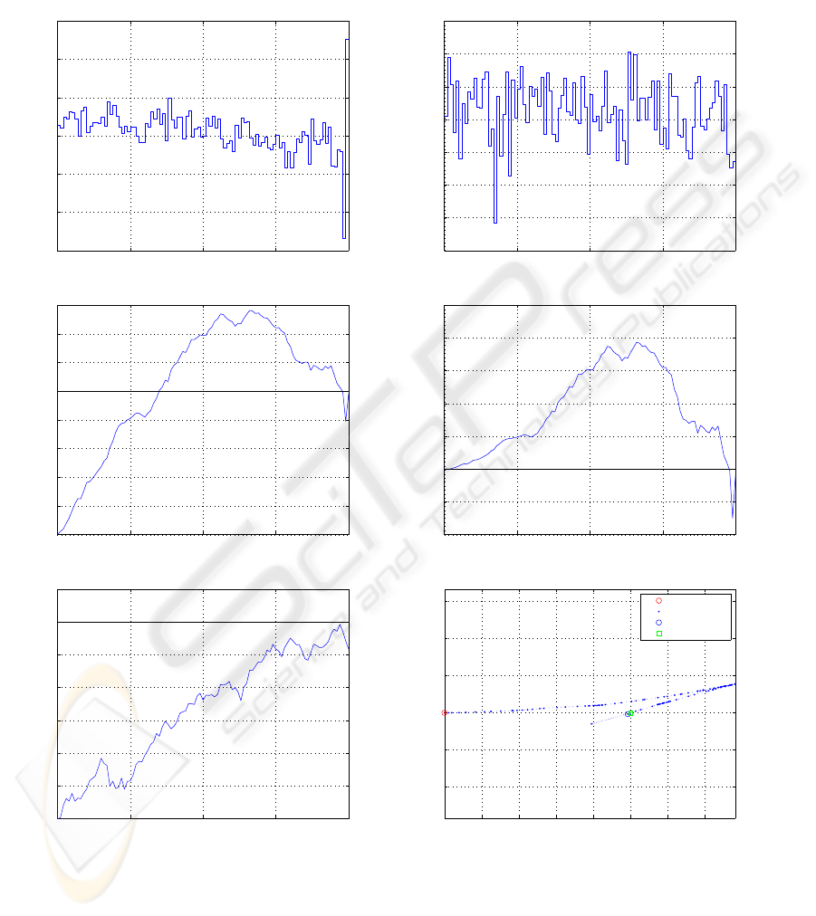
A Simulated path is presented in Figures 2: the
ideal simulated steer execution is perturbed by the
presence of some additive noise in the controls. This
simulate the effect of some non ideal controller be-
havior (wheel slipping, actuators dynamics, ...). The
constrained quadratic problems involved in the con-
trols computation are solved using an implementation
of the algorithm presented in (Coleman and Li, 1996)
5 CONCLUSION
In this paper, a kinematic model for a system com-
posed by a mobile robot and a camera, has been pre-
sented. Since such a model is exactly discretizable, it
has been possile to propose a multirate digital control
strategy able to steer the system to a desired pose in
an exact way. The effectiveness of the control scheme
adopted has been verified by simulations.
REFERENCES
Chelouah, A., Di Giamberardino, P., Monaco, S., and
Normand-Cyrot, D. (1993). Digital control of non-
holonomic systems two case studies. In Decision and
Control, 1993., Proceedings of the 32nd IEEE Con-
ference on, pages 2664–2669vol.3.
Chen, J., Dixon, W., Dawson, M., and McIntyre, M. (2006).
Homography-based visual servo tracking control of a
wheeled mobile robot. Robotics, IEEE Transactions
on [see also Robotics and Automation, IEEE Transac-
tions on], 22(2):406–415.
Coleman, T. and Li, Y. (1996). A reflective newton method
for minimizing a quadratic function subject to bounds
on some of the variables. SIAM Journal on Optimiza-
tion, 6(4):1040–1058.
Di Giamberardino, P. (2001). Control of nonlinear driftless
dynamics: continuous solutions from discrete time de-
sign. In Decision and Control, 2001. Proceedings of
the 40th IEEE Conference on, volume 2, pages 1731–
1736vol.2.
Di Giamberardino, P., Grassini, F., Monaco, S., and
Normand-Cyrot, D. (1996a). Piecewise continuous
control for a car-like robot: implementation and ex-
perimental results. In Decision and Control, 1996.,
Proceedings of the 35th IEEE, volume 3, pages 3564–
3569vol.3.
Di Giamberardino, P., Monaco, S., and Normand-Cyrot, D.
(1996b). Digital control through finite feedback dis-
cretizability. In Robotics and Automation, 1996. Pro-
ceedings., 1996 IEEE International Conference on,
volume 4, pages 3141–3146vol.4.
Lopez-Nicolas, G., Sagues, C., Guerrero, J., Kragic, D., and
Jensfelt, P. (2006). Nonholonomic epipolar visual ser-
voing. In Robotics and Automation, 2006. ICRA 2006.
Proceedings 2006 IEEE International Conference on,
pages 2378–2384.
Mariottini, G., Prattichizzo, D., and Oriolo, G. (2006).
Image-based visual servoing for nonholonomic mo-
bile robots with central catadioptric camera. In
Robotics and Automation, 2006. ICRA 2006. Proceed-
ings 2006 IEEE International Conference on, pages
538–544.
Monaco, S. and Normand-Cyrot, D. (1985). On the sam-
pling of a linear analytic control system. In Deci-
sion and Control, 1985., Proceedings of the 24th IEEE
Conference on, pages pp. 1457–1461.
Monaco, S. and Normand-Cyrot, D. (1992). An introduc-
tion to motion planning under multirate digital con-
trol. In Decision and Control, 1992., Proceedings of
the 31st IEEE Conference on, pages 1780–1785vol.2.
Monaco, S. and Normand-Cyrot, D. (2001). Issues on non-
linear digital control. European Journal of Control,
7(2-3).
R. Hartley, A. Z. (2003). Multiple View Geometry in Com-
puter Vision. Number ISBN: 0-521-54051-8. Cam-
bridge University Press.
HOMOGRAPHY-BASED MOBILE ROBOT MODELING FOR DIGITAL CONTROL IMPLEMENTATION
263

0 5 10 15 20
−6
−4
−2
0
2
4
6
time [s]
v [m/s]
Iterated−Planning Control ( r = 100 )
0 5 10 15 20
−0.2
−0.15
−0.1
−0.05
0
0.05
0.1
0.15
time [s]
w [rad/s]
Iterated−Planning Control ( r = 100 )
0 5 10 15 20
0
1
2
3
4
5
6
7
8
time [s]
Iterated−Planning Control ( r = 100 )
X [m]
0 5 10 15 20
−0.4
−0.2
0
0.2
0.4
0.6
0.8
1
time [s]
Iterated−Planning Control ( r = 100 )
Y [m]
0 5 10 15 20
0
0.05
0.1
0.15
0.2
0.25
0.3
0.35
time [s]
Iterated−Planning Control ( r = 100 )
Theta [rad]
0 1 2 3 4 5 6 7
−2
−1
0
1
2
3
X [m]
Y [m]
Iterated−Planning Control ( r = 100 )
Start Point
Via Points
End Point
Desired Pose
Figure 2: Multirate control simulation ( d = 1m ). Additive random noise on controls ( gaussian with std.dev. 0.5 and 0.05,
for v and ω respectively ).
ICINCO 2007 - International Conference on Informatics in Control, Automation and Robotics
264