ESTIMATION PROCESS FOR TIRE-ROAD FORCES AND VEHICLE

SIDESLIP ANGLE

Guillaume Baffet, Ali Charara

Heudiasyc Laboratory (UMR CNRS 6599), Universit

e de Technologie de Compi

egne

Centre de recherche Royallieu, BP20529 - 60205 Compi

egne, France

Daniel Lechner

INRETS-MA Laboratory (Department of Accident Mechanism Analysis)

Chemin de la Croix Blanche, 13300 Salon de Provence, France

Keywords:

State observers, vehicle dynamic, sideslip angle estimation, tire-force estimation, wheel cornering stiffness

estimation, linear adaptive force model.

Abstract:

This study focuses on the estimation of car dynamic variables for the improvement of vehicle safety, handling

characteristics and comfort. More speciﬁcally, a new estimation process is proposed to estimate longitudi-

nal/lateral tire-road forces, sideslip angle and wheel cornering stiffness. This method uses measurements from

currently-available standard sensors (yaw rate, longitudinal/lateral accelerations, steering angle and angular

wheel velocities). The estimation process is separated into two blocks: the ﬁrst block contains an observer

whose principal role is to calculate tire-road forces without a descriptive force model, while in the second block

an observer estimates sideslip angle and cornering stiffness with an adaptive tire-force model. The different

observers are based on an Extended Kalman Filter (EKF). The estimation process is applied and compared to

real experimental data, notably sideslip angle and wheel force measurements. Experimental results show the

accuracy and potential of the estimation process.

1 INTRODUCTION

The last few years have seen the emergence in cars

of active security systems to reduce dangerous situ-

ations for drivers. Among these active security sys-

tems, Anti-lock Braking Systems (ABS) and Elec-

tronic Stability Programs (ESP) signiﬁcantly reduce

the number of road accidents. However, these sys-

tems may improved if the dynamic potential of a car

is well known. For example, information on tire-road

friction means a better deﬁnition of potential trajec-

tories, and therefore a better management of vehicle

controls. Nowadays, certain fundamental data relat-

ing to vehicle-dynamics are not measurable in a stan-

dard car for both technical and economic reasons. As

a consequence, dynamic variables such as tire forces

and sideslip angle must be observed or estimated.

Vehicle-dynamic estimation has been widely dis-

cussed in the literature, e.g. ((Kiencke and Nielsen,

2000), (Ungoren et al., 2004), (Lechner, 2002),

(Stephant et al., 2006)). The vehicle-road system is

usually modeled by combining a vehicle model with

a tire-force model in one block. One particularity

of this study is to separate the estimation modeling

into two blocks (shown in ﬁgure 1), where the ﬁrst

block concerns the car body dynamic while the sec-

ond is devoted to the tire-road interface dynamic. The

Measurements: yaw rate, steering angle, lateral acceleration

longitudinal acceleration, angular wheel velocities

Extended Kalman Filter

Four-wheel vehicle model

Random walk force model

Extended Kalman Filter

Side-slip angle model

Linear adaptive force model

Longitudinal and lateral tire forces, yaw rate

Block 1

Block 2

Estimations : Longitudinal and lateral forces, sideslip angle,

yaw rate, cornering stiffness

Observer O1,4w :

Observer O2,LM :

Figure 1: Estimation process. Observers O

1,4w

and O

2,LAM

ﬁrst block contains an Extended Kalman Filter (de-

noted as O

1,4w

) constructed with a four-wheel vehicle

Baffet G., Charara A. and Lechner D. (2007).

ESTIMATION PROCESS FOR TIRE-ROAD FORCES AND VEHICLE SIDESLIP ANGLE.

In Proceedings of the Fourth International Conference on Informatics in Control, Automation and Robotics, pages 5-10

DOI: 10.5220/0001623900050010

 SciTePress

model and a random walk force model. The ﬁrst ob-

server O

1,4w

estimates longitudinal/lateral tire forces

and yaw rate, which are inputs to the observer in the

second block (denoted as O

2,LAM

). This second ob-

server is developed from a sideslip angle model and a

linear adaptive force model.

Some studies have described observers which take

road friction variations into account ((Lakehal-ayat

et al., 2006), (Rabhi et al., 2005), (Ray, 1997)). In

the works of (Lakehal-ayat et al., 2006) road fric-

tion is considered as a disturbance. Alternatively, as

in (Rabhi et al., 2005), the tire-force parameters are

identiﬁed with an observer, while in (Ray, 1997) tire

forces are modeled with an integrated random walk

model. In this study a linear adaptive tire force model

is proposed (in block 2) with an eye to studying road

friction variations.

The rest of the paper is organized as follows. The

second section describes the vehicle model and the

observer O

1,4w

(block 1). Next, the third section

presents the sideslip angle and cornering stiffness ob-

server (O

2,LAM

in block 2). In the fourth section an

observability analysis is performed. The ﬁfth section

provides experimental results: the two observers are

evaluated with respect to sideslip angle and tire force

measurements. Finally, concluding remarks are given

in section 6.

2 BLOCK 1: OBSERVER FOR

TIRE-ROAD FORCE

This section describes the ﬁrst observer O

1,4w

con-

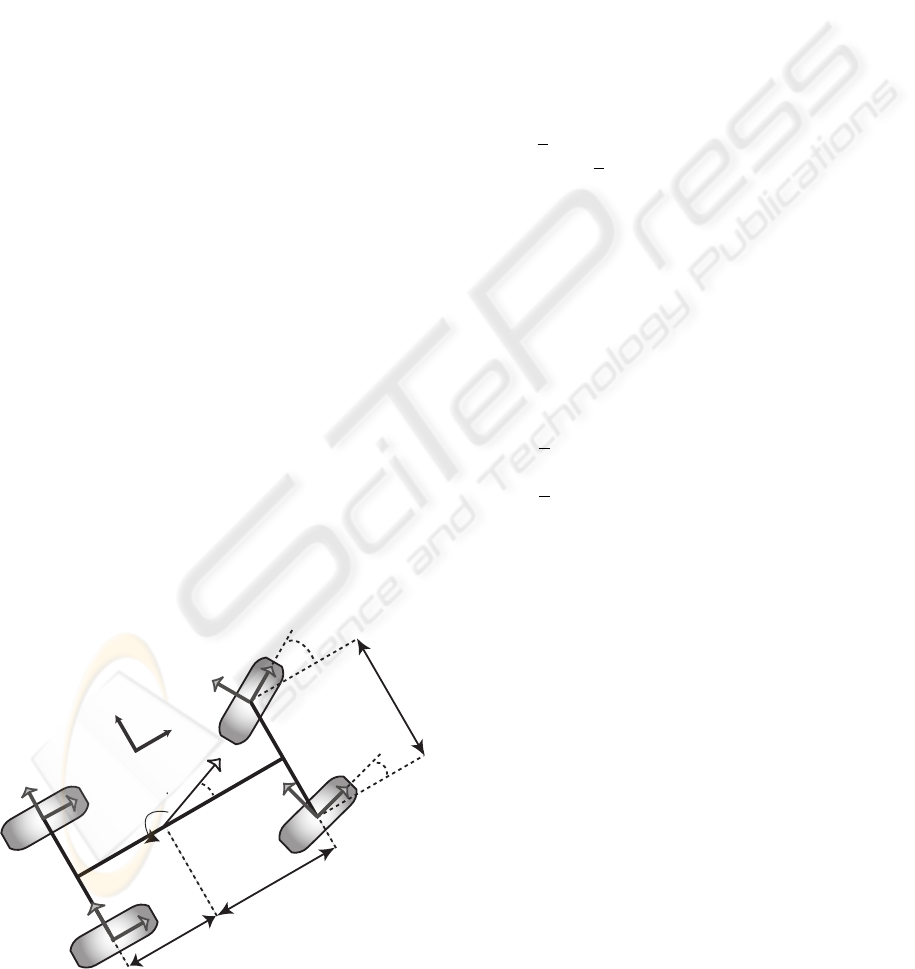
structed from a four-wheel vehicle model (ﬁgure 2),

where

ψ is the yaw rate, β the center of gravity

Fy21

Fx21

Fy22

Fx22

Fy12

δ2

Fx12

Fy11

δ1

Fx11

Fy11

Figure 2: Four-wheel vehicle model.

sideslip angle,V

the center of gravity velocity, and L

and L

the distance from the vehicle center of gravity

to the front and rear axles respectively. F

x,y,i, j

are the

longitudinal and lateral tire-road forces, δ

1,2

are the

front left and right steering angles respectively, and

E is the vehicle track (lateral distance from wheel to

wheel).

In order to develop an observable system (notably

in the case of null steering angles), rear longitudinal

forces are neglected relative to the front longitudinal

forces. The simpliﬁed equation for yaw acceleration

(four-wheel vehicle model) can be formulated as the

following dynamic relationship (O

1,4w

model):

ψ =







y11

cos(δ

) + F

y12

cos(δ

)

x11

sin(δ

) + F

x12

sin(δ

)]

−L

y21

+ F

y22

]

y11

sin(δ

) − F

y12

sin(δ

)

x12

cos(δ

) − F

x11

cos(δ

)]







, (1)

where m the vehicle mass and I

the yaw moment of

inertia. The different force evolutions are modeled

with a random walk model:

[

xij

yij

] = [0,0], i = 1, 2 j = 1, 2. (2)

The measurement vector Y and the measurement

model are:

Y = [

ψ,γ

,γ

] = [Y

ψ,

y11

cos(δ

) + F

y12

cos(δ

)

+(F

y21

+ F

y22

) + F

x11

sin(δ

) + F

x12

sin(δ

)],

[−F

y11

sin(δ

) − F

y12

sin(δ

)

x11

cos(δ

) + F

x12

cos(δ

)],

(3)

where γ

and γ

are the longitudinal and lateral accel-

erations respectively.

The O

1,4w

system (association between equations (1),

random walk force equation (2), and the measurement

equations (3)) is not observable in the case where

y21

and F

y22

are state vector components. For ex-

ample, in equation (1, 2, 3) there is no relation al-

lowing to distinguish the rear lateral forces F

y21

and

y22

in the sum (F

y21

y22

): as a consequence only

the sum (F

= F

y21

+ F

y22

) is observable. Moreover,

when driving in a straight line, yaw rate is small, δ

and δ

are approximately null, and hence there is no

signiﬁcant knowledge in equation (1, 2, 3) differenti-

ating F

y11

and F

y12

in the sum (F

y11

+ F

y12

), so only

the sum (F

= F

y11

+ F

y12

) is observable. These ob-

servations lead us to develop the O

1,4w

system with a

state vector composed of force sums:

X = [

ψ,F

], (4)

where F

is the sum of front longitudinal forces

= F

x11

x12

). Tire forces and force sums are as-

ICINCO 2007 - International Conference on Informatics in Control, Automation and Robotics

sociated according to the dispersion of vertical forces:

x11

z11

z12

+ F

z11

, F

x12

z12

+ F

z11

, (5)

y11

z11

z12

+ F

z11

, F

y12

z12

+ F

z11

, (6)

y21

z21

z22

+ F

z21

, F

y22

z22

+ F

z21

, (7)

where F

zij

are the vertical forces. These are calcu-

lated, neglecting roll and suspension movements, with

the following load transfer model:

z11

mg− h

cog

mγ

2(L

+ L

)

−

cog

mγ

+ L

, (8)

z12

mg− h

cog

mγ

2(L

+ L

)

cog

mγ

+ L

, (9)

z21

mg+ h

cog

mγ

2(L

+ L

)

−

cog

mγ

+ L

, (10)

z22

mg+ h

cog

mγ

2(L

+ L

)

cog

mγ

+ L

, (11)

cog

being the center of gravity height and g the grav-

itational constant. The load transfer model follows

the assumption of the superposition principle of in-

dependent longitudinal and lateral acceleration con-

tributions (Lechner, 2002). The input vectors U of

1,4w

observer is:

U = [δ

,δ

z11

z12

z21

z22

]. (12)

As regards the vertical force inputs, these are calcu-

lated from lateral and longitudinal accelerations with

the load transfer model.

3 BLOCK 2: OBSERVER FOR

SIDESLIP ANGLE AND

CORNERING STIFFNESS

This section presents the observer O

2,LAM

constructed

from a sideslip angle model and a tire-force model.

The sideslip angle model is based on the single-track

model (Segel, 1956), with neglected rear longitudinal

force:

β =

sin(δ− β) + F

cos(δ− β) + F

cos(β)

−

ψ.

(13)

Rear and front sideslip angles are calculated as:

= δ − β− L

ψ/V

= −β + L

ψ/V

(14)

where δ is the mean of front steering angles.

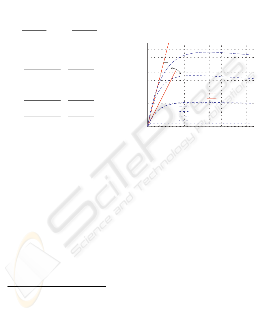
The dynamic of the tire-road contact is usually

formulated by modeling the tire-force as a function of

the slip between tire and road ((Pacejka and Bakker,

1991), (Kiencke and Nielsen, 2000), (Canudas-De-

Wit et al., 2003)). Figure 3 illustrates different lateral

tire-force models (linear, linear adaptive and Burck-

hardt for various road surfaces (Kiencke and Nielsen,

2000)). In this study lateral wheel slips are assumed to

be equal to the wheel sideslip angles. In current driv-

0 2 4 6 8 10 12 14 16

0.5

1.5

2.5

3.5

4.5

Front lateral slip, front wheel sideslip angle (°)

Front lateral tire force (kN)

Linear

Linear adaptive

Burckhardt, asphalt dry

Burckhardt, asphalt wet

Burckhardt, cobblestone wet

Burckhardt, ice

C1+∆Ca1

Figure 3: Lateral tire force models: linear, linear adaptive,

Burckhardt for various road surfaces.

ing situations, lateral tire forces may be considered

linear with respect to sideslip angle (linear model):

(β

) = C

, i = 1, 2, (15)

where C

is the wheel cornering stiffness, a parameter

closely related to tire-road friction.

When road friction changes or when the nonlinear

tire domain is reached, ”real” wheel cornering stiff-

ness varies. In order a take the wheel cornering stiff-

ness variations into account, we proposed an adaptive

tire-force model (named the linear adaptive tire-force

model, illustrated in ﬁgure 3). This model is based on

the linear model at which a readjustment variable ∆C

is added to correct wheel cornering stiffness errors:

(β

) = (C

+ ∆C

)β

. (16)

The variable ∆C

is included in the state vector of the

2,LAM

observer and it evolution equation is formu-

lated according to a random walk model (∆

= 0).

State X

′

∈R

, input U

′

∈R

and measurement Y

′

∈R

are chosen as:

′

= [x

′

] = [β, ∆C

,∆C

′

= [u

′

] = [δ,

ψ,V

′

= [y

′

] = [F

,γ

(17)

ESTIMATION PROCESS FOR TIRE-ROAD FORCES AND VEHICLE SIDESLIP ANGLE

The measurement model is

′

= (C

+ x

′

)β

′

= (C

+ x

′

)β

′

[(C

+ x

′

)β

cos(u

′

) + (C

+ x

′

)β

+ u

′

sin(u

′

)].

(18)

where

= u

′

− x

′

− L

′

= −x

′

+ L

′

(19)

Consider the state estimation denoted as

′

[

′

], the state evolution model of O

2,LAM

is:

′

sin(u

′

−

′

) + F

yw1,aux

cos(u

′

−

′

)

+ F

yw2,aux

cos(

′

)] − u

′

= 0,

′

= 0,

(20)

where the auxiliary variables F

yw1,aux

and F

yw2,aux

are

calculated as:

yw1,aux

= (C

′

)(u

′

−

′

− L

′

yw2,aux

= (C

′

)(−

′

+ L

′

(21)

4 OBSERVABILITY

The different observers (O

1,4w

, O

2,LAM

) were devel-

oped according to an extended Kalman ﬁlter method

(Kalman, 1960), (Mohinder and Angus, 1993).

The two observer systems are nonlinear, so the

two observability functions were calculated using

a lie derivative method (Nijmeijer and der Schaft,

1990). Ranks of the two observability functions cor-

responded to the state vector dimensions, so systems

1,4w

and O

2,LAM

were locally observable. Concern-

ing the observability of the complete systems (O

1,4w

and O

2,LAM

), a previous work (Baffet et al., 2006a)

showed that a similar system (in one block) is locally

observable.

5 EXPERIMENTAL RESULTS

The experimental vehicle (see ﬁgure 4) is a Peugeot

307 equipped with a number of sensors including

GPS, accelerometer, odometer, gyrometer, steering

angle, correvit and dynamometric hubs. Among these

sensors, the correvit (a non-contact optical sensor)

gives measurements of rear sideslip angle and vehi-

cle velocity, while the dynamometric hubs are wheel-

force transducers.

This study uses an experimental test representative

of both longitudinal and lateral dynamic behaviors.

Wheel-force transducers

Figure 4: Laboratory’s experimental vehicle.

The vehicle trajectory and the acceleration diagram

are shown in ﬁgure 5. During the test, the vehicle ﬁrst

accelerated up to γ

≈ 0.3g, then negotiated a slalom

at an approximate velocity of 12m/s (−0.6g < γ

0.6g), before ﬁnally decelerating to γ

≈ −0.7g. The

0 50 100 150

-1

Longitudinal position (m)

Lateral position (m)

-6 -4 -2 0 2

-5

Longitudinal acceleration (m/s )

acceleration

(m/s )

Lateral

Figure 5: Experimental test, vehicle positions, acceleration

diagram.

results are presented in two forms: ﬁgures of estima-

tions/measurements and tables of normalized errors.

The normalized error ε

for an estimation z is deﬁned

in (Stephant et al., 2006) as

= 100(kz− z

measurement

k)/(maxkz

measurement

k).

(22)

5.1 Block 1: Observer O

1,4w

Results

Figure 6 and table 1 present O

1,4w

observer results.

The state estimations were initialized using the max-

imum value of the measurements during the test (for

instance, the estimation of the front lateral force F

Table 1: Maximum absolute values, O

1,4w

normalized mean

errors and normalized standard deviation (Std).

maxkk Mean Std

5816 N 3.1% 4.0%

3782 N 2.9% 5.4%

9305 N 3.1% 4.1%

24.6

/s 0.4% 2.6%

ICINCO 2007 - International Conference on Informatics in Control, Automation and Robotics

0 5 10 15 20 25

-5

O1,4w, Front lateral tire force F

(kN)

0 5 10 15 20 25

-2

O1,4w, Rear lateral tire force F

(kN)

0 5 10 15 20 25

-10

-5

O1,4w, Front longitudinal tire force F

(kN)

Times (s)

Measurement

O1,4w

Measurement

O1,4w

Measurement

O1,4w

5155 N

Figure 6: Experimental test. O

1,4w

results in comparison

with measurements.

was set to 5155 N). In spite of these false initial-

izations the estimations converge quickly to the mea-

sured values, showing the good convergence proper-

ties of the observer. Moreover, the O

1,4w

observer

produces satisfactory estimations close to measure-

ments (normalized mean and standard deviations er-

rors are less than 7 %). These good experimental re-

sults conﬁrm that the observer approach may be an

appropriate way for the estimation of tire-forces.

5.2 Block 2: Observer O

2,LAM

Results

During the test, (F

) inputs of O

2,LAM

were

originally those from the O

1,4w

observer. The V

in-

put of O

2,LAM

was obtained from the wheel angular

velocities. In order to demonstrate the improvement

provided by the observer using the linear adaptive

force model (O

2,LAM

, equation 16), another observer

constructed with a linear ﬁxed force model is used

in comparison (denoted O

, equation 15, described

in (Baffet et al., 2006b)). The robustness of the two

observers is tested with respect to tire-road friction

variations by performing the tests with different cor-

nering stiffness parameters ([C

] ∗ 0.5,1, 1.5). The

observers were evaluated for the same test presented

in section 5.

Figure 7 shows the estimation results of observer O

for rear sideslip angle. Observer O

gives good re-

sults when cornering stiffnesses are approximately

known ([C

] ∗ 1). However, this observer is not

robust when cornering stiffnesses change ([C

] ∗

0.5,1.5).

0 5 10 15 20 25

-5

Orl, Rear Sideslip angle (°)

, C

)

, C

)*0.5

measurement

, C

)*1.5

Figure 7: Observer O

using a ﬁxed linear force model, rear

sideslip angle estimations with different cornering stiffness

settings.

Figure 8 and table 2 show estimation results for

the adaptive observer O

2,LAM

. The performance ro-

bustness of O

2,LAM

is very good, since sideslip angle

is well estimated irrespective of cornering stiffness

settings. This result is conﬁrmed by the normalized

mean errors (Table 2) which are approximately con-

stant (about 7 %). The front and rear cornering stiff-

ness estimations (C

+ ∆C

) converge quickly to the

same values after the beginning of the slalom at 12 s.

Table 2: Observer O

LAM

, rear sideslip angle estimation re-

sults, maximum absolute value, normalized mean errors.

2,LAM

0.5(C

) (C

) 1.5(C

)

maxkβ

k 3.0

3.0

Mean

7.4% 7.0% 7.2%

6 CONCLUSIONS AND FUTURE

WORK

This study deals with two vehicle-dynamic observers

constructed for use in a two-block estimation pro-

cess. Experimental results show that the ﬁrst observer

1,4w

gives force estimations close to the measure-

ments, and the second observer O

2,LAM

provides good

ESTIMATION PROCESS FOR TIRE-ROAD FORCES AND VEHICLE SIDESLIP ANGLE

0 5 10 15 20 25

-2

O2,LAM, Rear sideslip angle (°)

0 5 10 15 20 25

x 10

O2,LAM, Front cornering stiffness (N.rad

-1

)

0 5 10 15 20 25

x 10

O2,LAM, Rear cornering stiffness (N.rad

-1

)

, C

)*1.5

, C

)

, C

)*0.5

measurement

, C

)*1.5

, C

)*1.5

, C

)

, C

)*0.5

, C

)

, C

)*0.5

Figure 8: O

2,LAM

adaptive observer, Sideslip angle estima-

tion results, Front and rear cornering stiffness estimations

+ ∆C

, with different cornering stiffness settings.

sideslip angle estimations with good robustness prop-

erties relative to cornering stiffness changes. This re-

sult justiﬁes the use of an adaptive tire-force model to

take into account road friction changes.

Future studies will improve vehicle/road models in or-

der to widen validity domains for observers. Subse-

quent vehicle/road models will take into account roll

and vertical dynamics.

REFERENCES

Baffet, G., Stephant, J., and Charara, A. (2006a). Sideslip

angle lateral tire force and road friction estimation in

simulations and experiments. Proceedings of the IEEE

conference on control application CCA Munich Ger-

many.

Baffet, G., Stephant, J., and Charara, A. (2006b). Vehi-

cle sideslip angle and lateral tire-force estimations in

standard and critical driving situations: Simulations

and experiments. Proceedings of the 8th International

Symposium on Advanced Vehicle Control AVEC2006

Taipei Taiwan.

Canudas-De-Wit, C., Tsiotras, P., Velenis, E., Basset, M.,

and Gissinger, G. (2003). Dynamic friction models for

road/tire longitudinal interaction. volume 39, pages

189–226. Vehicle System Dynamics.

Kalman, R. E. (1960). A new approach to linear ﬁltering

and prediction problems. volume 82, pages 35–45.

Transactions of the ASME - PUBLISHER of Basic

Engineering.

Kiencke, U. and Nielsen, L. (2000). Automotive control

system. Springer.

Lakehal-ayat, M., Tseng, H. E., Mao, Y., and j. Karidas

(2006). Disturbance observer for lateral velocity es-

timation. Proceedings of the 8th International Sympo-

sium on Advanced Vehicle Control AVEC2006 Taipei

Taiwan.

Lechner, D. (2002). Analyse du comportement dynamique

des vehicules routiers legers: developpement d’une

methodologie appliquee a la securite primaire. Ph.D.

dissertation Ecole Centrale de Lyon France.

Mohinder, S. G. and Angus, P. A. (1993). Kalman ﬁltering

theory and practice. Prentice hall.

Nijmeijer, H. and der Schaft, A. J. V. (1990). Nonlinear

dynamical control systems. Springer-Verlag.

Pacejka, H. B. and Bakker, E. (1991). The magic formula

tyre model. pages 1–18. Int. colloq. on tyre models

for vehicle dynamics analysis.

Rabhi, A., M’Sirdi, N. K., Zbiri, N., and Delanne, Y.

(2005). Vehicle-road interaction modelling for esti-

mation of contact forces. volume 43, pages 403–411.

Vehicle System Dynamics.

Ray, L. (1997). Nonlinear tire force estimation and road

friction identiﬁcation : Simulation and experiments.

volume 33, pages 1819–1833. Automatica.

Segel, M. L. (1956). Theorical prediction and experimen-

tal substantiation of the response of the automobile to

steering control. volume 7, pages 310–330. automo-

bile division of the institut of mechanical engineers.

Stephant, J., Charara, A., and Meizel, D. (Available online 5

June 2006). Evaluation of a sliding mode observer for

vehicle sideslip angle. Control Engineering Practice.

Ungoren, A. Y., Peng, H., and Tseng, H. E. (2004). A study

on lateral speed estimation methods. volume 2, pages

126–144. Int. J. Vehicle Autonomous Systems.

ICINCO 2007 - International Conference on Informatics in Control, Automation and Robotics