TOWARDS A MULTIMODELING APPROACH

OF DYNAMIC SYSTEMS FOR DIAGNOSIS

Marc Le Goc and Emilie Masse

Laboratoire des Sciences de l'Information et des Systemes - LSIS, UMR CNRS 6168 - Paul Cezanne Aix-Marseille III

University, Avenue Escadrille Normandie Niemen, Marseille, France

Keywords: Modeling, Model Based Diagnosis, Dynamic Systems, Conceptual Model.

Abstract: This paper presents the basis of a multimodeling methodolog

y that uses a CommonKADS conceptual model

to interpret the diagnosis knowledge with the aim of representing the system with three models: a structural

model describing the relations between the components of the system, a functional model describing the

relations between the values the variables of the system can take (i.e. the functions) and a behavioural model

describing the states of the system and the discrete events firing the state transitions. The relation between

these models is made with the notion of variable: a variable used in a function of the functional model is

associated with an element of the structural model and a discrete event is defined as the affectation of a

value to a variable. This methodology is presented in this paper with a toy but pedagogic problem: the

technical diagnosis of a car. The motivating idea is that using the same level of abstraction that the expert

can facilitate the problem solving reasoning.

1 INTRODUCTION

This paper is concerned with the design of

knowledge based systems to supervise, diagnose and

control industrial process. The dynamic aspect of

industrial processes poses the difficult problem of

the acquisition and the representation of the

underlying temporal knowledge which is often

mixed with other types of knowledge (Basseville

and al, 1996).

To solve these problems, we first focus our

rks on the multi model based diagnosis approach

(Chittaro and al, 1993) with the aim of designing

models at the same level of abstraction level than the

experts. Second, we want that the model formalisms

to be adequate to represent the temporal knowledge

coming from both from Experts and from the

learning algorithms of the Stochastic Approach of

(Le Goc et al, 2005). And three, we want the

interpretation knowledge to closed to the cognitive

tasks the models are made for and we propose to use

a generic conceptual models. So, section 2 of this

paper positions shortly our approach according to

the main modelling approaches for diagnosis.

Section 3 presents the basis of our methodology

through its application to a toy but pedagogic

problem: the technical diagnosis of a car. Finally,

section 4 states our conclusions and perspectives.

2 MODELLING APPROACHES

The limitations and the problems (Dagues, 2001) of

the heuristic approach (Clancey, 1985) has

motivated the Model Based Diagnosis approach

(MBD) where the knowledge about the system is

represented in a unique logical model (Reiter, 1987).

The MBD approach use of a unique model of the

stem to be diagnosed containing the knowledge

about both the structure (components and

interconnections) and the behavior of the system

(relations between the values of the input and the

output of the components). This model generally

comes from the design model of the system so that it

contains a lot of components leading to

computational difficulties for the diagnosis task (the

number of potential diagnosis is exponential with the

number of components). This problem is crucial and

has motivate a large amount of works to reduce the

size of the space search. But more, this model

contains nothing about the evolution of the values of

the variables over time and nothing to represent the

knowledge about the state of the system. This is a

crucial lack when diagnosing a dynamic system

where the observations are timed.

The Multi Model Based Diagnosis (MMBD) has

been

proposed to avoid these problems (Chittaro and

al, 1993). This approach defines four models linked

277

Le Goc M. and Masse E. (2007).

TOWARDS A MULTIMODELING APPROACH OF DYNAMIC SYSTEMS FOR DIAGNOSIS.

In Proceedings of the Second International Conference on Software and Data Technologies - PL/DPS/KE/WsMUSE, pages 277-282

DOI: 10.5220/0001341702770282

 SciTePress

each other to describe the system to diagnose (cf.

(Zouaoui, 1998) and (Thetiot, 1999) for examples).

The first one is the Structural Model that describes

the components constituting the system and how

they are connected each other. The second model is

the Behavioral Model describing how components

work in terms of the physical laws linking quantities.

These two models represent the fundamental

knowledge. The third model is the Functional Model

describing the different roles the components may

play in the physical processes in which they take

part. The concept of function is the basis of the

description of the functional roles, the processes and

the phenomena that provides an interpretation of the

fundamental knowledge. The goals assigned to the

system by its designer(s) are described in the last

model, the Teleological Model. These two last

models refer to the interpretation knowledge.

Indeed, the MMBD is still concerned with the

computational problem of the diagnosis linked with

the number of the components declared in the

structural model (Zouaoui, 1998). This problem is

directly connected to the abstraction level which is

still defined by the designer(s).

3 MODELLING WITH EXPERTS

ASSUMPTIONS

So, our works is based on the hypothesis that an

expert uses a set of models at a level of abstraction

that allows efficient diagnosis reasoning and this

level of abstraction is directly linked with the

diagnosis task, not the design task.

We propose to use a CommonKADS conceptual

model (Schreiber and al, 2000) to interpret a

knowledge source with the aim of representing the

system with three models (Zanni and al, 2005): a

structural model describing the relations between the

components of the system, a functional model

describing the relations between the values the

variables can take (i.e. mathematical functions) and

a behavioural model describing the states of the

system (corresponding to the operating modes of

(Chittaro and al, 1993)) and the discrete events firing

the state transitions. The relation between these

models is made with the notion of variable: a

variable used in a function of the functional model is

associated with an element of the structural model

and a discrete event is defined as the affectation of a

value to a variable.

Left Node

Symbol

Relation

Symbol

Right Node

Symbol

Figure 1: Typical Binary Relation.

We define a model as an organized set of binary

relations B(S

, S

) between symbols S

denoting

objects described in the domain ontology of the

conceptual model of the knowledge. A binary

relation B(S

, S

) is also denoted with a symbol (i.e.

B). Such a binary relation only means that there exist

a link between the objects denoted with the symbols

and S

. A typical graphical representation of a

binary relation is provided in Figure 1, where nodes

are boxes or circles and the relation is eventually

represented with an ellipse. When useful, the arcs

can be oriented to show the orientation of a flow like

typically a flow of energy, material or information.

A model can then be represented with a graph

where nodes are symbols and arcs are relations.

Basically, a node symbol denotes a component or an

aggregate of components (i.e. a structure) in a

structural model, a variable in a functional model or

a state in a behavioural model. An arc represents a

link between two nodes. Such a link can be a

connection link between two structures in a

structural model, an information link between the

values of variables in a functional model or a

transition between two states in a behavioural

model. Consequently, a binary relation in a

structural model represents a connection between

two structures; a mathematical function in a

functional model and a transition between two states

in a behavioural model. It is to note that a set of

binary relations with the same right node symbol can

be aggregated in a single n-ary relation when this

aggregation is meaningful (an arithmetical function

between 3 variables for example).

Functional

Model

Behavioral

Model

Structural

Model

(Structure, Event)

(Variable, Event)

(Variable, Structure)

Functional

Model

Behavioral

Model

Structural

Model

(Structure, Event)

(Variable, Event)

(Variable, Structure)

Figure 2: Links between the three models.

With this simple formalism, a structural model is

an organised set of physical relations between

components or aggregates, a functional model is an

organised set of logical relations defining the values

of a variable given those of a set of variables, and a

behavioural model is a set of sequential relations

between states. These sequential relations can be

conditioned with predicates concerning the

occurrence of discrete events. A discrete event is

defined according to spatial discretization principle

of the Stochastic Approach (Le Goc et al, 2005) as a

couple (x, i) where x is a symbol denoting a variable

ICSOFT 2007 - International Conference on Software and Data Technologies

278

and i is a value for x so that a discrete event

occurrence is triplet (x, i, t

) meaning: x(t

)=i.

The modelling is based on three principles. The

first is that each object symbol S

used in one of the

three models denotes a concept that is defined at the

domain level of a CommonKADS model. This

means that the introduction of an object symbol that

is not associated with an element of the knowledge

domain model is prohibited. This model provides

then the means for interpreting the three models. The

second principle is that a variable is always

associated with a component or an aggregate defined

in the structural model. The values a variable can

take are provided either from its associated

components (input variable) or are computed with a

function defined in the functional model. And the

third principle is that a transition between two states

is conditioned either with the time elapsed in a state

(autonomous transition) or with a logical formula

linking the occurrences of discrete events. The

notion of variable constitutes then the common point

of the three models (Figure 2), providing a means to

the consistency analysis of the models.

Fuse

blown

Battery

low

Fuel Tank

empty

Fuse inspection

broken

Battery dial

low

Gas in engine

false

Power

off

Engine behavior

does not start

Engine behavior

stops

R1 R2 R3 R4 R6

Gas dial

zeo

R9R8

Figure 3: An example of a knowledge base.

4 APPLICATION

To illustrate the modelling process using these

principles, let us take the example providing from

(Schreiber et al, 2000) of the (simple) knowledge

base used to diagnose a car.

Figure 3 proposes a graphical representation of

the set R={R

, P

)} of the nine rules constituting

the knowledge base. In this graph, a rule R

, P

)

denote a logical consequence relation from a

proposition P

to another P

. This logical relation is

used to represent a causal relation between a cause

(Fuel Tank empty) and an effect (Gas in engine

false). To interpret this knowledge, we will use the

classical and minimal CommonKADS diagnosis

template «hypothesis generation and hypothesis

discrimination» (Zanni and al, 2005). This template

(Figure 4) considers the diagnosis reasoning as being

made of two basic inferences, one to generate the

hypothesis from the observed behaviour and the

second to discriminate between the different

hypotheses according to the observed behaviour.

hypothesis

observed behavior

generate hypothesis

discriminate hypothesis

diagnosis

hypothesis

observed behavior

generate hypothesis

discriminate hypothesis

diagnosis

Figure 4: The Diagnosis Template.

This template allows the classification of the

propositions contained in the knowledge base in a

set of observed behaviour (Fuse inspection broken,

Engine behaviour does not start, Engine behaviour

stops, Battery dial low and Gas dial zero) and a set

of hypothesis (Fuse blow, Battery low, Fuel Tank

empty, Power off and Gas in engine false). The

observed behaviour set contains the complains that

motivate the diagnosis reasoning (Engine behaviour

does not start, engine behaviour stops). This

functional classification of the propositions leads to

distinguish a first set of rules S1={R1, R4, R5} that

allows to observe unobservable states of the car

from the second set of rules S2={R2, R3, R6, R7, R8,

R9} that expresses the propagation of an

unobservable car state (Fuse blow, Battery low, Fuel

Tank empty ) to another unobservable car state

(Power off, Gas in engine false) and finally, to the

complains. So the propositions of R can be

interpreted as binary relations between a variable

(Fuel Tank for example) and a value (empty): each

proposition corresponds to a predicate

Equal(Variable, Value). Consequently, a rule is an

instantiation of a second order relation of the form

Cause(xi=v1, xj=v2) where the symbol “=” denotes

the predicate Equal, xi and xj denote a variable and

v1 and v2 two values. This relation means then that

there exist a logical relation between the fact xi=v1

and xj=v2 (i.e. a logical rule xi=v1⇒xj=v2) and

supposes that there exists a physical relation

between the variables xi and xj that is to say between

the components or the aggregates ci and cj the

variables xi and xj are linked with. The set X={xi} of

symbol variable associated with the set C={ci} of

symbol components can then be build, and the

knowledge base R can then be rewritten as follow:

•

R1: If x1=Blown Then x4=Broken

• R2: If x1=Blown Then x7=Off

• R3: If x2=Low Then x7=Off

• R4: If x2=Low Then x5=Low

• R5: If x3=Empty Then x6=Zero

• R6: If x3=Empty Then x8=False

• R7: If x7=Off Then x9=Does_not_start

• R8: If x8=False Then x9=Does_not_start

TOWARDS A MULTIMODELING APPROACH OF DYNAMIC SYSTEMS FOR DIAGNOSIS

279

• R9: If x8=False Then x9=Stops

From these items, a set of connection relations of

the form ConnectedTo(ci, cj) can be deduced and

represented in the structural model of figure 5. The

symbol components electric_alimentation and

gas_alimentation, respectively associated with the

variables Power and Gas_in_engine, denotes

abstract aggregates of components. Similarly, the set

of underlying rules xi=v1⇒xj=v2 can be deduced.

When defining the domain set of value for each

variables, each rule xi=v1⇒xj=v2 subsumes a

function of the form xj=f(xi) at least defined when

xi=v1 and xj=v2. When two functions xj=fi(xi) and

xj=fk(xk, xj) share the same output variable xj, a new

function xj=fj(xi, xk) can be defined. In the

functional model of figure 6, a rectangle (node)

specifies a variable name and an ellipse (relation)

specifies a function names. When the value set of

each variable xi can be defined, the set F={fi} of

functions fi can be entirely specified with tables of

values. When a value is missing, it is always

possible to define the missing value as the

complement of the known values. For example, the

value set of the variable x1 is {Blown, not_Blown}.

The tables of figure 7 are formulated independently

of the variables, when using the notation o(f) and i(f)

to denote the value of the output and the input of the

function “f”.

To introduce the behavioural model, let us

consider the variable x9 associated with the

aggregate c9 (engine). The value set of x9 is {Off,

On} where Off means either stops or does not start.

The complains x9=Off can then be interpreted as an

undesirable car state and so, the predicate x9=On

corresponds to the desirable car state “the car is

working”. According to the set of rules R, the car

stay in this state until the occurrence of a discrete

event No_power (x7=Off) or No_gas (x8=False). In

this case, the car transit from a state Working to a

state Out of Power or Out of Gas, which are by

definition two transient states. As soon as the inertia

will have no effect, the car will stops in a Failure

state. When the ignition key will be off, the car will

be in a Broken down state where x9=Off: a repairing

action is required to bring back the car in a normal

Stop state. This analysis leads to the behavioural

model of Figure 8, which is a finite state machine

represented with the DEVS formalism (Le Goc et al,

2006). This formalism is compatible with the

formalism of Figure 1: nodes (circles) are states and

links are state transitions. Autonomous transitions

(between Out of Gas and Failure) are represented

with dashed lines. An autonomous transition is fired

when the elapse time in a state qi is greater than the

maximum duration ΔTi of the qi state.

electric_

alimentation

gas_

alimentation

engine

gas_dial

battery_dial

fuse_inspection

fuse

battery

fuel_tank

R8 and R9

Figure 5: Structural model.

Figure 6: Functional model.

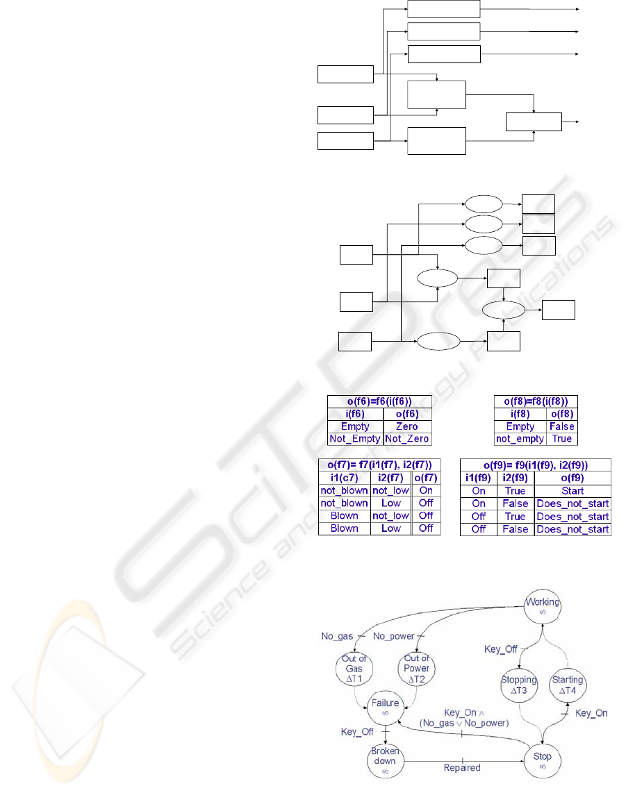
Figure 7: Specification of the functions.

Figure 8: Behavioural model.

The models of figures 5, 6, 7 and 8 are implicitly

contained in the initial knowledge base of figure 3,

ICSOFT 2007 - International Conference on Software and Data Technologies

280

but the behavioural model is the most “covered”.

Such an observation is very frequent because the

dynamic properties are generally misunderstood. For

example, the difference between the values stops

and does not start becomes clear only when

considering the role of the ignition key in the

behavioural model. It is to note also that the

behavioural model is made of two parts: one part (at

the right of figure 8) describes the normal working

of the car (Working, Stop, Starting and Stopping

states), and the second part (at the left of figure 8)

describes the abnormal working of the car. Such a

notion can not be defined with the functional model

because it is defined as an organized set of relations

between values of variables. This means that when

considering dynamic systems, the normal

behavioural model notion of Reiter’s diagnosis

theory for static systems has been shifted in the

classification of the system states in normal and

abnormal categories. This leads to design a new

algorithm for diagnosing dynamic systems.

(f7)= f7(i1(f7), i2(f7

)

i1(c7) i2(f7) o(f7)

TTT

TFF

FTF

FFF

Figure 9: The f

function as an “AND” function

5 USING THE MODELS

The structural and functional models of figures 5, 6

and 7 can be used in Reiter’s diagnosis theory with a

simple logical transcription in the first order

predicate logic. The set of components COMPS is

deduced from the structural model:

COMPS={c1, c2,

c3, c4, c5, c6, c7, c8}

Figure 10: The nine rules as a logical circuit.

The system description SD is deduced from the

functional model when associating each function f

with the component c

corresponding to the output

variable of the function f

. For example, the function

is associated with the component c

through the

variable x

: x

=o(f

). Next, the symbols used to

specify the functions f

must be represented with the

Boolean symbols T for True and F for False. For

example, when rewritten the symbols not_Blown,

not_Low and Off as T and the symbols Blown, Low

and Off as F, the function f

become the logical

function AND (Figure 9). The same is true for the

functions f

and f

. Finaly, when considering the

components c

, c

and c

as sensors that can not

failed, this lead to consider the following logical

circuit of Figure 10. The system description is then:

SD = {

¬AN(x)∧FUSE(x) ⇒ o(x)=Not_blown,

¬AN(x)∧BATTERY(x) ⇒ o(x)=Not_low,

¬AN(x)∧FUEL_TANK(x) ⇒ o(x)=Not_Empty,

¬AN(x)∧AND_GATE(x) ⇒ o(x)=AND(i1(x), i2(x)),

//Component type declaration

FUSE(c1), BATTERY(c2), FUEL_TANK(c3),

AND_GATE(c7), AND_GATE(c8), AND_GATE (c9),

//Connexions

o(c1)=i1(c7), o(c2)=i2(c7), o(c3)=i1(c8), o(c3)=i2(c8),

o(c7)=i1(c9), o(c8)=i2(c9)

}

This model is not efficient for diagnosing

because, given the observations engine behaviour

stops or engine behaviour does not start, all the six

components will be suspected. Adding observation

as Gas dial zero reduces the problem, but to the

three components c7, c8 and c9, which can be

abnormal also.

Now, let us suppose that at time t

, the system is

in the Working state (Figure 8). The observation Gas

dial zero will be represented with the discrete event

occurrence (t

, x

, zero) (i.e. x

)=zero). The

functional model provides the relations: x

) and

). Given the functional model (figures 6 and

7), x

)=zero implies x

)=empty and x

)=false corresponding to the occurrence of the

discrete event No_gas, where

and

are the time

transfer of functions f

and f

. The behavioural

model of Figure 8 shows then that the system will

transit from state Working to the state Out of gas at

time t

, and finally in the state Failure at time

+ΔT

. So, if at time t

, the observation

engine behaviour stops is made on the car with t

≈t

+ΔT

, the observation Gas dial zero at time t

can be used to infer that the cause of this complain is

the fact that the fuel tank is empty since t

This example shows that a diagnosis algorithms

adapted to the reasoning with timed observations is

required. The difficulty of this problem can be

perceived trough the formulae “t

≈t

+ΔT

”.

The symbol ≈ denotes a temporal equality predicate

that is generally interpreted as the fact that the time

belongs to a timed interval containing the time “t

+ΔT

”. The basic but fundamental problem is

then to define these intervals. The Stochastic

Approach for learning timed relations between

discrete events proposes a solution to this problem

TOWARDS A MULTIMODELING APPROACH OF DYNAMIC SYSTEMS FOR DIAGNOSIS

281

(Le Goc and al, 2005). This is the reason why one of

the main requirements for our modelling approach is

to be compatible with this approach of learning.

6 CONCLUSION

This paper presents the basis of a multimodeling

methodology that uses a CommonKADS conceptual

model to interpret the knowledge source with the

aim of representing the system with three models: a

structural model describing the relations between the

components of the system, a functional model

describing the relations between the values the

variables of the system can take (i.e. the functions)

and a behavioral model describing the states of the

system and the discrete events firing the state

transitions. The relation between these models is

made with the notion of variable: a variable used in

a function of the functional model is associated with

an element of the structural model and a discrete

event is defined as the affectation of a value to a

variable.

This methodology is presented in this paper with

a toy but pedagogic problem: the technical diagnosis

of a car with a given knowledge base (Schreiber and

al, 2000). This example shows that the resulting

models are compatible with Reiter’s theory of

diagnosis and that a specific reasoning is required to

take advantage of the behavioural model of the

dynamic system to diagnose. Such reasoning must

take into account the time of the observations. This

example illustrates clearly our goal: making explicit

the models used by experts to formulate their

knowledge. The idea is that using the same level of

abstraction that the expert can facilitate the problem

solving reasoning. This method has been applied to a

real world dynamic system, the Cubblize dam,

confirming the conclusions presented in this paper

and validating the method (Masse and Le Goc,

2007). It is to note finally that the resulting models

can be used either fore the design or the simulation

phases.

Our current work aims at formalizing the global

methodology and to design of a diagnosis algorithm

able to use a behavioural model that can be built

according to the timed relation the Stochastic

Approach of knowledge learning discovers.

REFERENCES

Basseville, M. and Cordier, M-O., 1996. Surveillance et

diagnostic de systèmes dynamiques : approches

complémentaires du traitement de signal et de

l’intelligence artificielle, office publication.

Bouché, P., Le Goc, M., and Giambiasi, N., 2005.

Modeling Discrete Event Sequences for Discovering

Diagnosis Signatures, Summer Computer Simulation

Conference, SCSC'05, Philadelphia, USA.

Clancey, W., 1985. Heuristic classification, Artificial

Intelligence Journal 25(3) 289-350.

Cordier, M.O., Dousson, C., 2000. « Alarm driven

monitoring based on chronicles », Proceedings of

SafeProcess 2000, pp.286-291, Budapest, Hungary.

Chittaro, L., Guida, G., Tasso, C., and Toppano, E., 1993.

Functional and teleological knowledge in the

multimodeling approach for reasoning about physical

systems: a case study in diagnosis. IEEE transactions

on systems.

Dagues, P., 2001. « Théorie logique du diagnostic à base

de modèles », in Diagnostic, intelligence artificielle et

reconnaissance des formes, Hermes, p. 17-105.

Le Goc, M., Bouché, P. and Giambiasi, N., 2005.

Stochastic modeling of continuous time discrete event

sequence for diagnosis. Proceedings of the 16th

International Workshop on Principles of Diagnosis,

DX-05, Pacific Grove, California, USA.

Le Goc, M., Bouché, P., Giambiasi, N., 2006. DEVS, a

formalism to operationnalize chronicle models in the

ELP Laboratory. Proceedings of DEVS’06, DEVS

Integrative M&S Symposium, Part of the 2006 Spring

Simulation Multiconference (SpringSim'06), pp. 143-

150, Van Braun Convention, Huntsville, Alabama,

USA, April 2-6 2006.

Masse, E., and Le Goc, M., 2007. Modeling Dynamic

Systems from their Behavior for a Multi Model Based

Diagnosis. To appear in the proceedings of the 18th

International Workshop on the Principles of Diagnosis

(DX‘07), Nashville, USA, Mai 29th to 31th 2007.

Reiter, R., 1987. A theory for Diagnosis from First

Principles, Artificial Intelligence 32, P 57-95.

Schreiber, A. Th., Akkermans, J. M., Anjewierden, A. A.,

de Hoog, R., Shadbolt, N. R., Van de Velde W.,

Wielinga B. J., 2000. Publication, Knowledge

Engineering and Management, The CommonKADS

methodology, MIT Press.

Thetiot, R., 1999. PhD in Sciences, Utilisation de

l’approche multi-modèles pour l’aide au diagnostic

d’installations industrielles, Université d’Evry Val d’

Essonne.

Zanni, C., Le Goc, M., Frydman, C., 2005. Publication, A

conceptual framework for the analysis, Classification

and choice of knowledge-based diagnosis systems,

International Journal of Knowledge-Based &

Intelligent Engineering Systems (KES Journal), IOS

Press Eds., 41 p.

Zouaoui, F., 1998. PhD in Sciences, Aide à

l’interprétation du fonctionnement des systèmes phy-

siques en utilisant une approche multi-modèles.

Application au circuit primaire d’une centrale à eau

pressurisée, Université de Paris XI – Orsay.

ICSOFT 2007 - International Conference on Software and Data Technologies

282