ADJACENT CHANNEL INTERFERENCE

Impact on the Capacity of WCDMA/FDD Networks

Daniel Figueiredo, Pedro Matos, Nuno Cota, António Rodrigues

Instituto Superior Técnico, Technical University of Lisbon, Av. Rovisco Pais, Lisbon, Portugal

Keywords: WCDMA, adjacent channel interference (ACI), FDD, spectrum management

Abstract: The adjacent channel interference (ACI) can result in a reduced network capacity in a multioperator

WCDMA/FDD environment. This paper is devoted to the study of the ACI, using a static simulator.

Simulations were performed in order to identify particular scenarios and network compositions where ACI

plays a major role in the system capacity. On the basis of the results, the authors identify the best strategy

for frequency deployment within the available spectrum. It is demonstrated that the macro carrier should be

located in the centre of the frequency band, protected from the ACI introduced by other operators. It is, in

fact, the carrier which suffers the greatest losses caused by the increase in ACI. Furthermore, the micro

carrier should be placed as close as possible to the adjacent channel of other operators in order to maximize

system capacity.

1 INTRODUCTION

At the moment radio spectrum is becoming

increasingly more occupied, making its

management a vital tool to network planning. It is

under these circumstances that the third generation

(3G) mobile communications systems emerged, and

in particular the UMTS (Universal Mobile

Telecommunications System) in Europe. The air

interface chosen for the 3G UMTS system was

WCDMA (Wideband Code Division Multiple

Access) for the paired bands FDD (Frequency

Division Duplex). The scope of this paper is to

study the impact of frequency utilization on

WCDMA/FDD networks and develop a strategy to

optimise it.

The performance of any CDMA system is

conditioned by the interference. From the various

possible sources of interference that are present in

these systems this paper focuses on the study of

adjacent channel interference (ACI) and its effect

on the overall capacity of the system.

This study consists of five main sections.

Following a brief overview of a few features of

UMTS related with the options chosen for the

simulations, to be found in Section 2, the criteria for

the choice of the tested scenarios are explained in

Section 3. Section 4 presents the results obtained

with the simulated scenarios, and final conclusions

are drawn in Section 5.

2 INTERFERENCE ISSUES IN

UMTS/FDD NETWORKS

When defining the UMTS system, 3GPP (3

Generation Partnership Project) inferred that each

radio channel has a bandwidth of 5 MHz and the

channels allocated are positioned beside each other

in uplink and downlink bands separated by 190

MHz (3GPP 25.101). Each channel has its carrier

and these are assigned to the UMTS operators in the

market.

The strategy designed to reduce the

interference, thus achieving the highest possible

capacity, consists in identifying optimal spacing

between carriers in the radio spectrum available for

use. For this purpose, a specific frequency

arrangement must be considered, as it may vary

from country to country.

The initial licensed spectrum for UMTS in

FDD mode was a band with twelve carriers, both

uplink and downlink. The case considered includes

four operators, each of which has been allocated

three carriers. Within the allocated band, it is

Figueiredo D., Matos P., Cota N. and Rodrigues A. (2004).

ADJACENT CHANNEL INTERFERENCE - Impact on the Capacity of WCDMA/FDD Networks.

In Proceedings of the First International Conference on E-Business and Telecommunication Networks, pages 74-80

DOI: 10.5220/0001381900740080

 SciTePress

possible to choose the spacing between its carriers

and the distance from adjacent operator carriers.

3GPP defines for the spacing between channels a

raster of 200 kHz (3GPP 25.104), which means that

the spacing between carriers can vary in increments

of 200 kHz around 5 MHz.

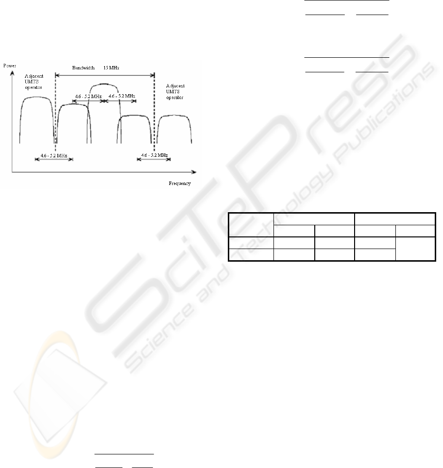
As seen in Figure 1, in order to decide which

spacing should be used, more issues must be taken

into account, to prevent the carriers from

encroaching on their neighbours. Consequently,

bearing in mind the limits typically used in

simulations, it has been chosen to vary the distances

between the values 4.6 and 5.2 MHz.

Figure 1: Spacing between carriers in a UMTS system

(adapted from (Holma and Toskala, 2002))

In a WCDMA system, developed in the above

context, the interference can stem from a large

number of sources, namely, thermal noise, traffic in

the same cell, traffic in adjacent cells and traffic

from operators using adjacent cells.

Possible ways of measuring the interference

leakage between connections operating on different

carriers must be considered. As the filter is not

perfect, when transmitting in its own channel, one

carrier will send part of its power into adjacent

channels. This effect is measured as the ACLR

(Adjacent Channel Leakage Ratio). On the other

hand, the receiver filter is unable to receive only the

desired signal alone, which is why the rejection of

the adjacent channel signal is measured as ACS

(Adjacent Channel Selectivity). Moreover, when

considering the existence of two carriers which

interfering with each other, the total interference is

given as an ACIR (Adjacent Channel Interference

Ratio) and determined by (1).

(1)

CLR

ACIR

Furthermore, this source of interference can be

seen both from the uplink and from the downlink

standpoint. Consider an uplink connection, whose

ACIR is given in (2) below. As it is quite likely that

the filter in the user equipment (UE) will be poorer

than the filter in the base station (BS), the UE

ACLR dominates in the case of uplink. In

downlink, the situation is analogous, as seen in (3),

where the UE ACS dominating on this occasion.

(2)

BSUE

ACSACLR

ACIR

(3)

UEBS

ACSACLR

ACIR

One of the essential parameters used in the

simulation was that the value of the filter depends

on the spacing given to the channels. 3GPP defines

the filter’s mask, while identifying minimum values

for filters at 5 and 10 MHz [3, 4]. However, in this

project more realistic values were used, which

correspond to real equipment presently available.

These values may be found in Table 1.

Table 1: Values of the filters used in BS and UE

ACLR (dB) ACS (dB) Spacing

(MHz)

UE BS UE BS

5 33 60 33

10 43 65 43

When simulations were run using spacing

different from 5 or 10 MHz, e.g. 4.6 MHz, a

logarithmic regression is made to convert the filter

value and obtain a valid method to compare the

results.

3 SIMULATION SCENARIOS

The choice of which scenarios to study was not as

simple as it might be assumed at first glance. One of

the goals in this paper was to find scenarios where

ACI has a major role on the network’s capacity, in

order to understand the impact of placing carriers

with different spacing. In (3GPP 25.942), the

authors give an idea of the issues to be born in mind

when choosing which scenarios to simulate.

In a preliminary stage, the search started with

the study of the representative scenarios of rural and

urban environments. When simulating two

operators, BSs working with adjacent carriers were

uniformly distributed over a map. In order to

ADJACENT CHANNEL INTERFERENCE - Impact on the Capacity of WCDMA/FDD Networks

simulate a worst case situation, the sites of both

operators are not co-located and the interoperator

spatial offset is equal to the cell radius (Hiltunen,

2002).

It was found that the inter-frequency

interference impact on the capacity was minimal,

when compared with the intra-frequency

interference. The reason for this result lies in the

fact that there are too many BSs from the same

carrier interfering with each other.

The next step taken was to identify scenarios

where the ACI played a significant role, at least as

important as the interference coming from the

connections working on the same carrier. Following

simple scenarios, where just a few BSs and two

carriers were taken into account, the analysis

developed to encompass broader environments

simulating urban centres with many antenna sites

and three carriers.

A simple map was used as an entrance

parameter to the simulator, with no additional

information, apart from UE and BS positions. When

placing the BSs of two different carriers, one must

decide whether they are co-located, i.e. both cells

lie on the same site, or not. In the latter situation, it

is assumed that the worst case for ACI happens, i.e.

the adjacent channel site is located at the coverage

edge of the first channel cell.

The simulator used to achieve this analysis was

static, using a Monte-Carlo evaluation method. As a

result, the users were placed randomly on the map.

Following the iterative process, only the

connections with sufficient Eb/No (or signal to

noise ratio - SNR) for the appointed service were

considered to be served by the system. This

simulator was adapted from the previous one

described in (Laiho et al., 2002) and (Wacker et al.,

2001). By examining many static situations,

referred to as snapshots, network capacity is

estimated through the average number of the served

users (Povey et al., 2003).

The bit rates tested in this study were chosen in

accordance with the services expected to be offered

by operators in the first implementation phase. In

this case, 12.2 kbps with CS (Circuit Switching), 64

kbps with CS and, finally, 128 kbps in downlink

and 64 kbps in uplink using PS (Packet Switching).

The results are presented taking into account users

accessing one of these three types of services.

The UE power classes considered for

determining the maximum output power were class

3 (24 dBm) for voice and class 4 (21 dBm) for data

services (3GPP 25.101). The BS maximum output

power used was 43 dBm.

Two types of antennas were chosen to simulate

macro and micro BS: for the macro BS, tri-

sectorized antennas with 18 dBi of gain, and for the

micro BS, omni-directional antennas with 4 dBi of

gain.

Two different propagation models were

considered to calculate the path loss according to

the characteristics of the environment (both for

outdoor propagation). For rural scenarios the COST

231 Hata model was used. The main input

parameters for the model are the UE antenna

heights, 1.5 m, and BS antenna heights, 35 m. For

the urban environment the propagation model

applied was COST 231 Walfish-Ikegami. The main

parameters used are UE antenna heights, 1.5 m, BS

antenna heights, between 10 and 25 m (depending if

they are macro or micro), street width, 20 m,

building separation, 40 m, and building height, 12

4 RESULTS

In the extended study that originated this paper, a

wide range of scenarios and environments were

considered (Figueiredo and Matos, 2003). Urban,

rural and motorway environment were tested using

layers containing twenty-three macro cells placed in

the form of a grid. Furthermore, eight scenarios

with only a few antennas (five at the most) were run

to simulate specific situations using macro and

micro cells. The dense urban environment was

simulated, by using macro cells layers and micro

cells to cover identified hotspots. In this paper, only

the three most significant tests will be presented.

At the end of each simulation, the outputs were

analysed. Apart from the maps indicating the BS

and UE position, the network’s capacity (measured

in average number of served users) and the capacity

loss (when compared with no ACI), parameters like

the ratio between sources of interference were also

analysed in (Figueiredo and Matos, 2003). The

interference sources considered in the results

included the interference coming from the adjacent

channel, the interference from the same channel

from neighbouring cells and the interference from

the same cell (due to the other users connected to

the same BS).

A maximum load of 50 % was allowed in the

radio interface.

4.1 Case 1: Small scale networks with

two operators

This scenario was developed to study the impact of

a new micro BS placed by an operator to cover a

hotspot in the middle of an existing network of

macro BSs from the adjacent carrier competitor.

ICETE 2004 - WIRELESS COMMUNICATION SYSTEMS AND NETWORKS

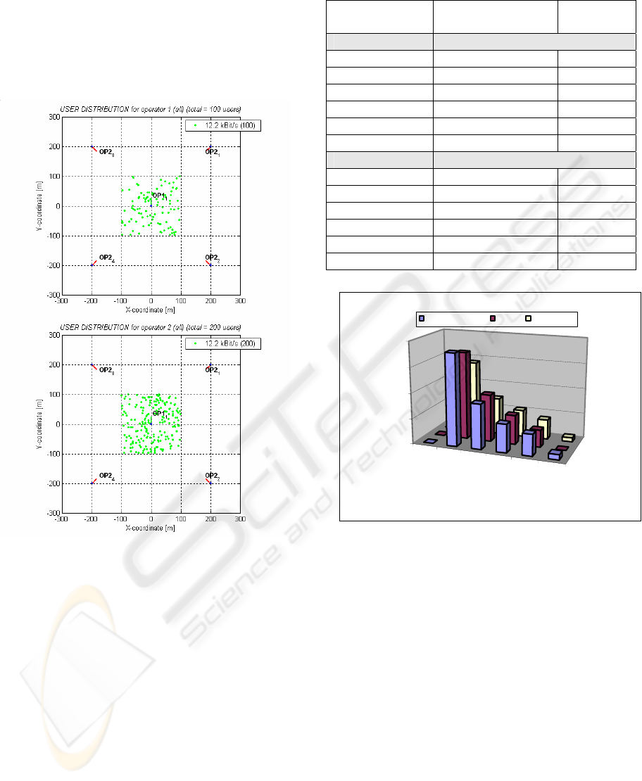
The users from both operators have been located

around the centre of the area considered. The area

simulated has a high density of active clients, as

shown in Figure 2.

The number of users presented in Figure 2

corresponds to the initial users from each operator,

and are placed on the map at the simulation start.

Figure 2: Location of UE (CS 12.2) and BS (Case 1)

Table 2 shows the average number of users

served employing different channel spacing and the

percentage of loss compared to the case where no

adjacent operator exists (without ACI) for the CS

12.2 kbps service.

It has been verified that the operator 2,

covering the area with four macro BSs, is the one

that suffers most from interference. This may be

explained by the fact that users of operator 1 (micro

BS) are closer to the antenna, which therefore

makes it more difficult for them to lose the

connection. A comparison of the results obtained

from the simulations performed with the three

services tested for operator 2, is shown in the graph

presented in Figure 3.

Table 2: Results from the simulated scenario (Case 1)

CS 12.2 kbps Capacity (average

number of users)

Capacity

Loss (%)

Operator 1

Without ACI

77 0

4.6 MHz

76.1 1.17

4.8 MHz

75.8 1.56

5.0 MHz

76.7 0.39

5.2 MHz

76.7 0.39

10.0 MHz

77 0

Operator 2

Without ACI

162.1 0

4.6 MHz

44.8 72.36

4.8 MHz

104.7 35.41

5.0 MHz

126.2 22.15

5.2 MHz

134.6 16.96

10.0 MHz

155.5 4.07

Without ACI

4.6 MHz

4.8 MHz

5.0 MHz

5.2 MHz

10 MHz

Capacity Loss (%)

Spacing between carriers

Scenario from case 1

CS 12.2 (Voice) CS 64 PS 64/128

Figure 3: Capacity Loss of operator 2 (Case 1)

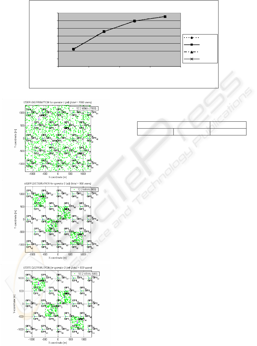
4.2 Case 2: One layer macro and two

layers micro

In the situation shown in Figure 5 several macro

BSs were placed to form a grid and cover the area

to serve users of operator 1. Four hotspot areas

(with higher user density) from both operators 1 and

2 were placed and micro BSs located to cover them.

In this case, it has been tested an environment

where three carriers coexist and interfere with each

other. Operator 1 has one carrier for macro BSs (f1)

and another for micro BSs (f2). Operator 2 has only

one carrier for micro BSs (f3). The three channels

were allocated next to each other in the radio

spectrum as shown in Table 3.

ADJACENT CHANNEL INTERFERENCE - Impact on the Capacity of WCDMA/FDD Networks

Scenario from case 2

1200

1250

1300

1350

1400

1450

1500

1550

4.6 MHz 4.8 MHz 5 MHz 5.2 MHz

Spacing betw een carriers macro and micro from operator 1

Average number of served

users by operator 1

4.6 MH

4.8 MH

5 MHz

5.2 MH

Figure 4: Capacity of operator 1 (Case 2)

Figure 5: Location of UE (CS 12.2) and BS (Case 2)

Table 3: Frequency planning with macro (M) and micro

(m) networks (Case 2)

Operator 1 Operator 2

f1 (M) f2 (m) f3 (m)

Once again the spacing considered between

each of the three channels varied within the range

4.6 to 5.2 MHz.

The results obtained from these simulations are

given in Figure 4. The graph shows the average

number of users served by operator 1, and take into

account both the users connected to the macro (f1)

and to the micro (f2) layers. As expected, it can be

seen that the network capacity rises when the

spacing between f1 and f2 widens. As both micro

layers accommodate fewer users than the macro

layer from operator 1, it is evident that the distance

between micro layers (f2 and f3) from the different

operators does not have a great impact on the

capacity of operator 1. This fact is confirmed by the

graph, since the lines are almost overlapped.

Following the analysis of these results, it is

logically preferable to choose a wider spacing

between carriers f1 and f2, in order to achieve an

increase in the capacity of operator 1. At the same

time, it is reasonable to leave the lowest distance to

the carrier from operator 2 (f3), since the damage is

imperceptible, towards optimisation of the spectrum

allocated.

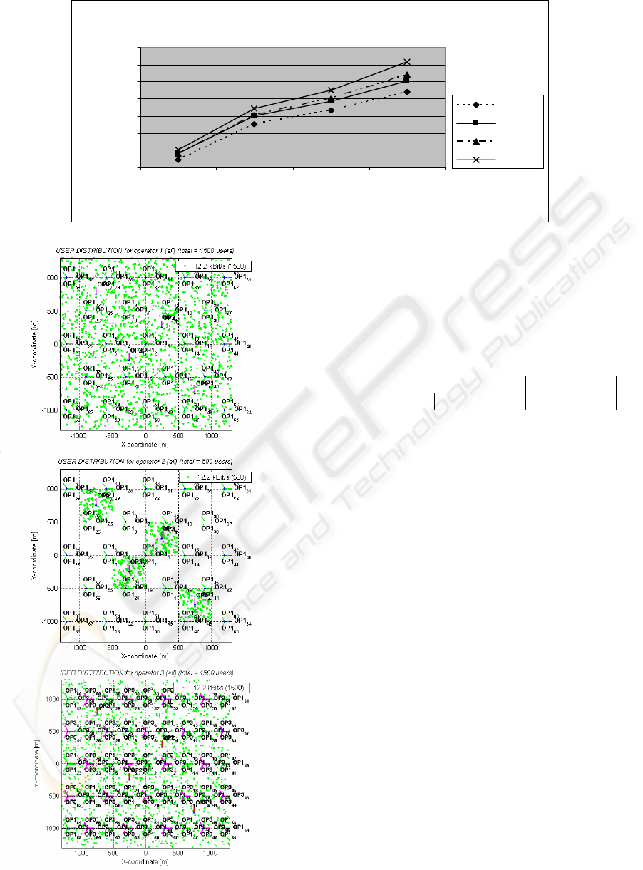
4.3 Case 3: Two layers macro and

one layer micro

As in the previous case, in Case 3, the authors

tested the impact of interference among three

carriers controlled by two operators. However, in

this case, there are two major macro BSs grids from

operators 1 and 2. The same hotspots mentioned in

Spacing between

erators 1 and 2

ICETE 2004 - WIRELESS COMMUNICATION SYSTEMS AND NETWORKS

Scenario from case 3

1200

1250

1300

1350

1400

1450

1500

1550

4.6 MHz 4.8 MHz 5 MHz 5.2 MHz

Spacing betw een carriers f1 and f 2 f rom operator 1

Aaverage number of users

served by operator 1

4.6 MHz

4.8 MHz

5 MHz

5.2 MHz

Figure 6: Capacity of operator 1 (Case 3)

Figure 7: Location of UE (CS 12.2) and BS (Case 3)

Case 2 are now covered with micro BSs by operator

1 only, as seen in Figure 7. Thus, the configuration

of the radio spectrum is similar, the only difference

being that there are two channels for macro BSs and

one for micro BSs, as shown in Table 4.

Table 4: Frequency planning with macro (M) and micro

(m) networks (Case 3)

Operator 1 Operator 2

f1 (M) f2 (m) f3 (M)

The results, presented in the graph from Figure

6, were obtained by using the same procedure

followed in Case 2.

As before, the network’s capacity grows as the

distance between f1 and f2 becomes larger.

However, it can now be confirmed that the spacing

between the two adjacent carriers from different

operators (f2 and f3) has a significant impact on the

overall capacity of operator 1. This feature is due to

the fact that carrier f3, from operator 2, now

accommodates a much larger number of users in its

macro layer.

In this situation the analysis has to be

considered more carefully than in the previous case.

To achieve maximum capacity in operator 1,

apparently the best solution would be to choose the

maximum spacing between carriers f1 and f2

whilst, at the same time, also leaving the highest

distance to the adjacent operator channel (f3).

However, in doing so, one is failing to take into

account the fact that each operator has three

allocated channels. Note that, in the future, it will

be valuable to use all of them to face an anticipated

traffic increase. As a result, it would wise to choose

a configuration in which the two carriers from

operator 1 are not positioned in such a way that they

occupy the free space left by hitherto unused third

channel.

Spacing between

erato

s 1 and 2

ADJACENT CHANNEL INTERFERENCE - Impact on the Capacity of WCDMA/FDD Networks

5 CONCLUSIONS

In this paper the authors studied the impact of the

ACI on a general network’s capacity. This led to

some more useful conclusions that may be applied

when planning the launch of a WCDMA/FDD radio

networks.

When considering two wide BSs grids that lie

close to each other to cover a specific area, it was

observed that the main interference source is not the

ACI, but interference from the neighbouring BSs,

working on the same channel.

From scenarios like the one presented in Case

1, it was noted that the macro BSs are more likely

to suffer from ACI when new hotspots are covered

with micro BS by a competitor operator. This fact is

explained by the longer distance between the user

and the macro BS, as compared with the latter. As

the macro carrier may suffer a greater impact on

capacity, it should be protected and placed in the

centre channel of the allocated spectrum. This

choice is irrespective of the number or type of

carriers used, assuming that the operator launching

a service uses at least one macro carrier.

It may also be seen, from these small and

specific case scenarios like Case 1, that the use of a

4.6 MHz spacing may cause critical problems,

leading to a serious reduction in the network’s

capacity. Therefore, distances between carriers of

4.6 MHz or less should never be used. Although in

the vast majority of the situations the loss may not

be that disastrous, the possibility of having certain

areas with losses above 50 % is unsustainable to an

operator.

Upon considering an available spectrum of

three carriers, and assuming that the macro carrier is

located in the centre channel, it is intended to

decide where to place the micro channel. From Case

2, where operator 2 placed a micro carrier in the

channel adjacent to the spectrum of operator 1, it

was seen that the distance between the two channels

was almost irrelevant to the overall network’s

capacity. However, when operator 2 has a macro

carrier on the channel, adjacent to operator 1, the

latter suffers the consequences of a reduction in the

distance between different operators’ channels. On

the basis of the compromise solution of not

occupying the spectrum of the three channels

allocated using two carriers only, it may be

concluded that a spacing of 5.2 MHz between f1

and f2 and 4.8 MHz between f2 and f3 is the best

option.

ACKNOWLEDGEMENTS

We would like to thank Luís Santo and Ana Claro

for their support and useful discussions that helped

to improve this work. The authors are also grateful

to Optimus for the support given to this project.

REFERENCES

Laiho, J., Wacker, A., and Novosad, T., 2002, Radio

Network Planning and Optimisation for UMTS, John

Wiley & Sons, Sussex, England

Holma, H., and Toskala, A., 2002, WCDMA for UMTS –

Edition, John Wiley & Sons, Sussex, England

3GPP Technical Specification 25.101 v5.5.0, UE Radio

Transmission and Reception (FDD)

3GPP Technical Specification 25.104 v5.5.0, BS Radio

Transmission and Reception (FDD)

3GPP Technical Specification 25.942 v5.1.0, Radio

Frequency (RF) System Scenarios

Hiltunen, K.,2002, Interference in WCDMA Multi-

Operator Environments, Postgraduate Course in

Radio Communications 2002-2003, Helsinki

University of Technology, Finland

Wacker, A., Laiho, J., Sipilä, K., Heiska, K., and

Heikkinen, 2001, K., NPSW – MatLab

Implementation of a Static Radio Network Planning

Tool for Wideband CDMA

Povey, G., Gatzoulis, L., Stewart, L., and Band, I., 2003,

WCDMA Inter-operator Interference and “Dead

Zones”, Elektrobit (UK) Ltd, University of Edinburgh

Figueiredo, D., and Matos, P., 2003, Analysis, Impact and

Strategy of Frequency Utilisation on WCDMA/FDD

Networks (in Portuguese), Final Graduation Thesis,

Instituto Superior Técnico, Lisboa, Portugal

ICETE 2004 - WIRELESS COMMUNICATION SYSTEMS AND NETWORKS