ACTIVE SENSING STRATEGIES FOR ROBOTIC PLATFORMS,
WITH AN APPLICATION IN VISION-BASED GRIPPING
Benjamin Deutsch
∗
, Frank Deinzer
∗
, Matthias Zobel
∗
Chair for Pattern Recognition, University of Erlangen-Nuremberg
91058 Erlangen, Germany
Joachim Denzler
Chair for Computer Vision, University of Passau
94030 Passau, Germany
Keywords:
Service Robotics, Object Tracking, Zoom Planning, Object Recognition, Grip Planning
Abstract:
We present a vision-based robotic system which uses a combination of several active sensing strategies to grip
a free-standing small target object with an initially unknown position and orientation. The object position is
determined and maintained with a probabilistic visual tracking system. The cameras on the robot contain a
motorized zoom lens, allowing the focal lengths of the cameras to be adjusted during the approach. Our system
uses an entropy-based approach to find the optimal zoom levels for reducing the uncertainty in the position
estimation in real-time. The object can only be gripped efficiently from a few distinct directions, requiring
the robot to first determine the pose of the object in a classification step, and then decide on the correct
angle of approach in a grip planning step. The optimal angle is trained and selected using reinforcement
learning, requiring no user-supplied knowledge about the object. The system is evaluated by comparing the
experimental results to ground-truth information.
1 INTRODUCTION
This paper focuses on the task of visual tracking, clas-
sification and gripping of a free-standing object by a
robot. Typically, vision-based robotic gripping ap-
plications (Smith and Papanikolopoulos, 1996), use
a passive, non-adaptive vision system. We present a
system which combines several active sensing strate-
gies to improve the sensor input available to the robot,
and allow the robot to choose the best approach direc-
tion. A quantitative evaluation of the robot’s perfor-
mance is achieved by comparing ground-truth infor-
mation with experimental results.
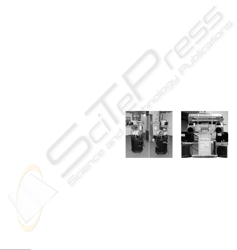
Our robot (see figure 1) consists of a platform with
a holonomic movement system, a stereo camera sys-
tem mounted on a pan-tilt-unit on top of the platform,
and a lift-like gripper on the front of the platform.
The object tracking subsystem uses the stereo head to
estimate the 3D position of the object relative to the
robot; this information is used to continuously adapt
the robot’s movement and guide it to the target. Ad-
ditionally, the two cameras possess motorized zoom
lenses, allowing the cameras’ zoom levels to be ad-
justed during tracking. Instead of a simple reactive
∗
This work was partly funded by the German Research
Foundation (DFG) under grant SFB 603/TP B2. Only the
authors are responsible for the content.
Figure 1: (left) Our robot, showing the stereo head and the
gripper (holding a plastic bottle). (right) The stereo head.
approach (Tordoff and Murray, 2001), or a trained
model-dependent behavior (Paletta and Pinz, 2000),
the tracking system automatically calculates the op-
timal zoom level with an entropy-based information
theoretical approach (Denzler and Brown, 2002).
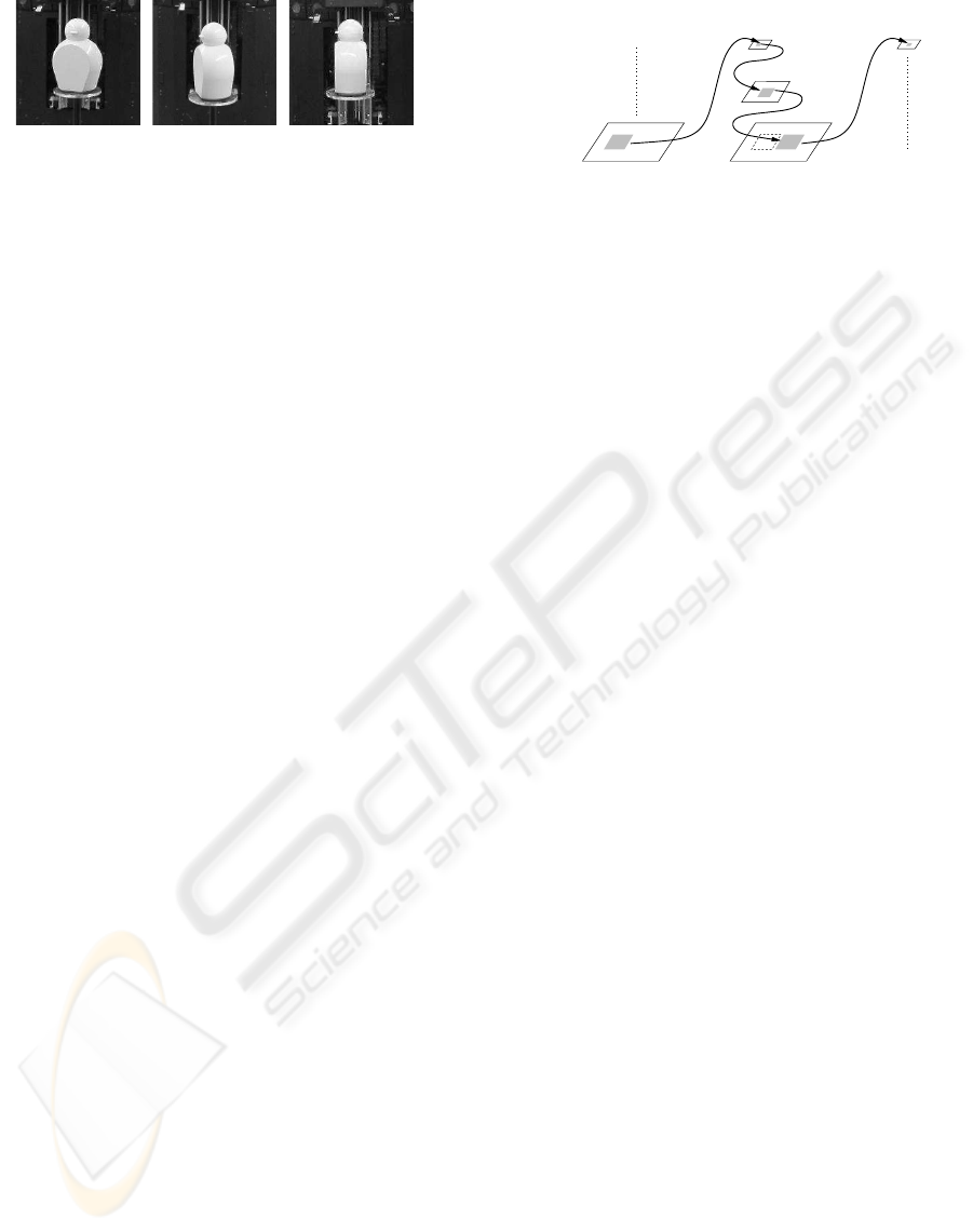
Since the objects used may not be gripped from ev-
ery angle (see figure 2 for examples of object orienta-
tion), the robot needs to detect the relative orientation
of the object and adjust its approach accordingly. The
object classifier generates both class and pose infor-
mation, of which only the latter is used in this system.
The gripping planner uses the pose information to
calculate the optimal gripping direction and the move-
ment the robot must perform to approach the object
169
Deutsch B., Deinzer F., Zobel M. and Denzler J. (2004).
ACTIVE SENSING STRATEGIES FOR ROBOTIC PLATFORMS, WITH AN APPLICATION IN VISION-BASED GRIPPING.
In Proceedings of the First International Conference on Informatics in Control, Automation and Robotics, pages 169-176
DOI: 10.5220/0001140901690176
Copyright
c
 SciTePress

PSfrag replacements
(a) (b) (c)
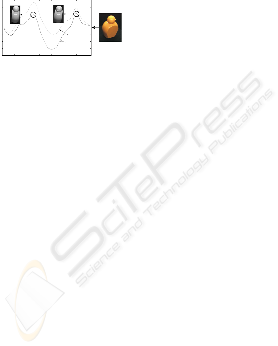
Figure 2: (a) An invalid gripping angle. (b) The worst still
acceptable gripping angle. (c) The optimal gripping angle.
from this direction. This is related to active viewpoint
selection for object recognition (Borotschnig et al.,
2000). The viable grabbing positions were not input
directly into the system; rather, the robot underwent a
training phase, using reinforcement learning.
It should be noted that, unlike robot grip planning
work as described in (Mason, 2001) or (Bicchi and
Kumar, 2000), determining the optimal gripping po-
sition from the shape, outline or silhouette of the ob-
ject is not a focus of our work. Instead, the optimal
gripping position is learned during the training phase
through feedback. This feedback could come from
successful or unsuccessful gripping attempts, or even
(as in our case) from a human judge. The robot can
generalize from this training and evaluate new, un-
trained gripping positions.
The rest of this paper is organized as follows: Sec-
tion 2 details the methods used for object tracking,
object classification and grip planning. It also shows
the interdependencies between the different subsys-
tems. Section 3 contains some experimental results.
It explains the exact setup that was used, the mea-
surements taken, and evaluates the results. Section
4 concludes this paper, and outlines future enhance-
ments which aim to enable the system to grip moving
targets as well.
2 METHODS
This section details the methods used in our system.
Section 2.1 describes the object tracker, section 2.2
the object classifier and grip planner, and section 2.3
the co-integration of the two.
2.1 Object Tracking
The purpose of the object tracking system is to deter-
mine the target object’s location relative to the robot
at all times. This information is critical for the robot’s
approach and the classification system (see section
2.2). The location is the 3D position of the target (x,
y and z coordinates in mm) relative to the stereo head.
The vision system consists of two cameras on a
pan-tilt unit with a vergence axis per camera (see fig-
ure 1 (right)). The pan axis is not used, leaving both
PSfrag replacements
Time step t − 1 t t + 1
Level 0
Level 1
Level 2
0
µ(t − 1)
2
µ(t)
1
µ(t)
0
µ(t)
Figure 3: The hierarchical extension to the region tracker.
cameras a shared tilt and individual vergence axes.
The object is first visually tracked in the cam-
era images with two 2D template-based object track-
ers, based on a system presented by (Hager and Bel-
humeur, 1998). A detailed description of the tracker
is beyond the scope of this paper; it is only necessary
to note that the tracker generates a time-dependant
motion parameter estimate µ(t), describing the mo-
tion of the tracked object in the image. The estimate
µ(t−1) from the previous time step is used as a start-
ing point for determining µ(t). The tracking system
on our robot uses motion parameters which describe
only translations in the image plane u and a relative
scaling factor s; these are sufficient for tracking a sta-
tionary object, given the planar robot movement.
One problem of the original implementation is that
it can only handle small object motions. Too large
motions will cause the trackers to lose the object. To
allow the object to move farther in the camera image
per time step, the tracker used in our system contains
a hierarchical extension (Zobel et al., 2002).
An image pyramid is created by scaling the camera
image and the reference template downwards k − 1
times, creating k levels of hierarchy. Typically, each
level has half the resolution of the one below it.
Each of these k levels then runs its own region
based tracker, scaled appropriately. Whereas the non-
hierarchical tracker uses the motion parameter esti-
mate µ(t − 1) as an initial value while tracking the
object from time step t−1 to time step t, the hierarchi-
cal tracker propagates the previous estimate through
its different levels. The initial estimate is still the
motion parameter vector
0
µ(t − 1) from level 0 of
the previous time step. However, it is now passed to
the tracker operating on level k − 1, the highest level,
which results in a (rough) estimate
k−1
µ(t). This is
then propagated down to level k − 2 and so on, the
last level receiving the estimate
1
µ(t) and calculating
the estimate
0
µ(t). Figure 3 shows an example with
3 hierarchy levels.
Using this scheme, the complete tracker can han-
dle larger movements, typically 2
k−1
times as large,
while still producing results just as accurate as the
non-hierarchical version. Of course, care needs to
be taken to scale the motion parameters between dif-
ferent levels; in our case of doubling resolutions, the
translation parameter u needs to be divided by 2
k−1
ICINCO 2004 - ROBOTICS AND AUTOMATION
170

when going from
0
µ(t − 1) to
k−1
µ(t), and multi-
plied by 2 for each descended level from there on.
The scaling parameter s is resolution independent and
does not need to be adjusted.
In our system, we use k = 3 hierarchy levels, pro-
viding a good compromise between tracking capabil-
ity and computation time requirements.
In order to combine, and smooth, the noisy 2D in-
formation provided by the two trackers, an extended
Kalman filter (Bar-Shalom and Fortmann, 1988) is
employed. The (extended) Kalman filter is a standard
state estimation tool and will not be described here. A
brief overview of the notation used here follows.
The object’s true state at time t is denoted by q
t
.
This is a 9-dimensional vector comprised of the 3D
position, velocity and acceleration of the object. For
each time step, the filter receives an observation o
t
(comprised, in our case, of four scalar values: the x
and y image coordinates of the target centers in the
two camera images) and incorporates this into its cur-
rent belief. The filter’s belief about the true state at
time t is a probability density function p(q
t
|hoi
t
),
where hoi
t
denotes all observations received up to
time t. In the case of the Kalman filter, this is as-
sumed to be a normal distribution N (
ˆ
q
+
t
, P
+
t
). The
filter uses a state transition model to predict a new
state estimate p(q
t+1
|q
t
) = N (
ˆ
q
−
t+1
, P
−
t+1
) from the
previous estimate. Upon receiving the next observa-
tion o
t+1
, the filter compares this to a predicted ob-
servation and updates its belief to p(q
t+1
|hoi
t+1
).
During the tracking process, it is possible to ad-
just the focal lengths of the cameras. It is clear that
such an adjustment will have an effect on the observa-
tion function used in the Kalman filter. This adds an
action parameter a to the object state belief, giving
p(q
t
|hoi
t
, hai
t
). The goal of the zoom planning sub-
system is to find an action a
∗
(in our case two zoom
levels, that is, the field-of-view of each camera) that is
optimal for the Kalman filter, i.e. one that minimizes
the uncertainty of the positional belief generated in
the next time step.
In the Kalman filter, this uncertainty is described by
the a-posteriori covariance matrix P
+
. The “larger”
the covariance matrix is, the more likely the true state
is deemed to be farther away from the estimated mean
ˆ
q
+
. Several different measurements for the covari-
ance matrix have been proposed in the context of es-
timation evaluation (Puckelsheim, 1993), such as the
determinant of the matrix, or the inverse of the trail of
its inverse (D- and A-Optimality, respectively).
Following (Denzler et al., 2003), we employ the
entropy of the posterior distribution as an uncertainty
measure (Shannon, 1948). The entropy of the a-
posteriori density p(q
t
|hoi
t
, hai
t
) is defined as
H(q) = −
Z
p(q
t
|hoi
t
, hai
t
) log p(q
t
|hoi
t
, hai
t
)dq
t
.
(1)
Since (for our system) p(q
t
|hoi
t
, hai
t
) is an n-
dimensional normal distribution N (
ˆ
q
+
, P
+
), the en-
tropy can be calculated as
H(q) =
n
2
+
1
2
log
¡
(2π)
n
|P
+
|
¢
(2)
Unfortunately, the correct entropy can only be calcu-
lated after the most recent observation o
t
has taken
place, yet we wish to choose an action a
t
based on
this entropy before the observation. What we need to
calculate is the conditional entropy
H(q
t
|o
t
, a
t
) =
Z
p(o
t
|a
t
)H(q
t
)do
t
. (3)
This is, in effect, the expected entropy of the belief
over all observations o
t
, given the action a
t
. In the
case of the Kalman filter, P
+
is independent of the
actual observation o
t
. Using this information and re-
moving all terms which are irrelevant to the optimiza-
tion, we obtain
a
∗
t
= arg min
a
t
|P
+
t
| (4)
There is one problem with this approach, however:
this formula assumes that there will always be an ob-
servation, no matter how large the focal length. This
is clearly not always the case. One of the main prob-
lems with a large focal length is the associated small
field of view. A larger focal length increases the
chance that the object’s projection will in fact be out-
side of a camera’s sensor. In this case, no (usable)
observation has occurred, and the best estimate for
the object’s current state is the a-priori state estimate
p(q
t
|hqi
t−1
, hoi
t−1
) = N (
ˆ
q
−
t
, P
−
t
).
Splitting the conditional entropy into successful
and unsuccessful observations, an unsuccessful obser-
vation being an observation which lies outside one of
the camera’s sensors, one can define w
1
(a
t
) to be the
chance that the object will be visible and the observa-
tion will be successful, and w
2
(a
t
) as the chance that
the object will not be visible (Denzler et al., 2003).
w
1
(a
t
) and w
2
(a
t
) can be estimated using Monte
Carlo sampling, or by closed-form evaluation in the
case of normal distributions.
Although any irrelevant terms for the optimization
can still be eliminated, the logarithms can no longer
be avoided. This leaves the optimization problem
a
∗
t
= arg min
a
t
³
w
1
(a
t
) log
¡
|P
+
t
(a
t
)|
¢
+ w
2
(a
t
) log
¡
|P
−
t
|
¢
´
(5)
2.2 Object Classification — Grip
Planning
One of the goals of this work is to provide a solution
to the problem of selecting an optimal grippoint resp.
ACTIVE SENSING STRATEGIES FOR ROBOTIC PLATFORMS, WITH AN APPLICATION IN VISION-BASED
GRIPPING
171

PSfrag replacements
Mobile platform,
classifier
Grip planning
Action a
t
State s
t
Reward r
t
r
t+1
s
t+1
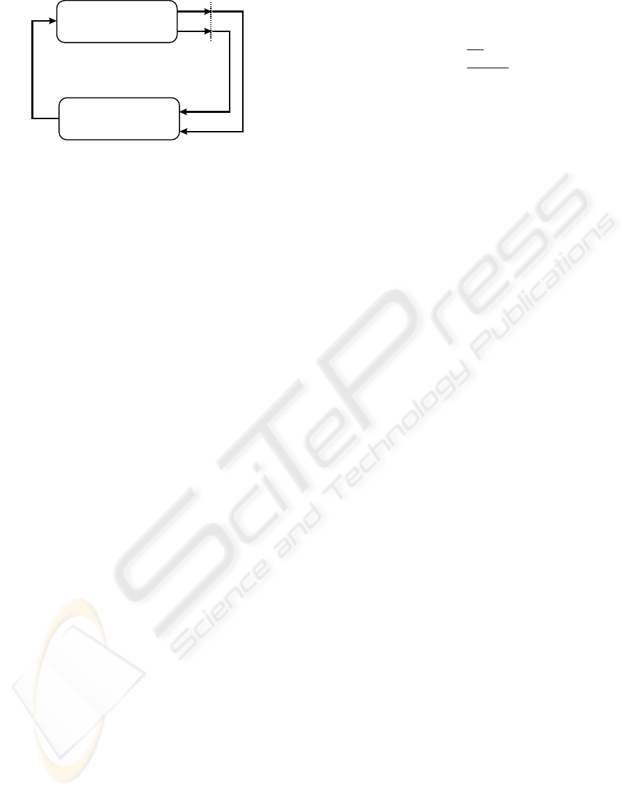
Figure 4: Principles of Reinforcement Learning applied to
grip planning.
grip positions without making a priori assumptions
about the objects and the classifier used to recognize
the class and pose of the object. The problem is to
determine the next view of an object given the current
observations. The problem can also be seen as the de-
termination of a function which maps an observation
to a new grippoint. This function should be estimated
automatically during a training step and should fur-
ther improve over time. The estimation must be done
by defining a criterion, which measures how good it
is to grip an object from a specific position. Addition-
ally, the function should take uncertainty into account
in the recognition process as well as in the grippoint
selection. The latter one is important, since the robot
must move around the object to reach the planned
grippoint; a noisy operation. So the final position of
the robot will always be error-prone. Last not least,
the function should be classifier independent and be
able to handle continuous grippoints.
A straight forward and intuitive way to formalizing
the problem is given by looking at figure 4. A closed
loop between sensing s
t
and acting a
t
can be seen.
The chosen action
a
t
= (∆ϕ) with ∆ϕ ∈ [0
◦
; 360
◦
[ (6)
corresponds to the movement of the mobile platform.
As it will only move on a circle around the object in
the application presented in this paper, the definition
of (6) is sufficient. The sensed state
s
t
= (Ω
κ
, ϕ)
T
with ϕ ∈ [0
◦
; 360
◦
[ (7)
contains the class Ω
κ
and pose ϕ (the rotation) of the
object relative to the robot. This state is estimated
by the employed classifier. In this paper we use a
wavelet-based classifier as described in (Grzegorzek
et al., 2003) but other classification approaches can
be applied. Additionally, a so called reward r
t
, which
measures the quality of the chosen grippoint is re-
quired. The better the chosen direction for gripping
an object, the higher the yielding reward has to be. In
our case we decided for r
t
∈ [0; MAX], MAX = 10
with r
t
= 0 for the worst grip position (figure 2(a))
and r
t
= 10 for the best grip position (figure 2(c)).
It is important to notice that the reward should also
include costs for the robot movement, so that large
movements of the robot are punished. These costs
cost(a) =
½
m · MAX ·
∆ϕ
360
∆ϕ ≤ 180
m · MAX ·
360−∆ϕ
360
∆ϕ > 180
(8)
with m ∈ [0; 1] are subtracted from each reward.
At time t during the decision process, the goal will
be to maximize the accumulated and weighted future
rewards, called the return
R
t
=
∞
X
n=0
γ
n
r
t+n+1
(9)
with γ ∈ [0; 1]. The weight γ defines how much in-
fluence a future reward will have on the overall return
R
t
at time t + n + 1. For the application of selecting
the optimal grip position γ = 0 is sufficient as only
one step is necessary to reach the goal, the optimal
grip position.
Of course, the future rewards cannot be observed at
time step t. Thus, the following function, called the
action-value function
Q(s, a) = E {R
t
|s
t
= s, a
t
= a} (10)
is defined, which describes the expected return when
starting at time step t in state s with action a. In
other words, the function Q(s, a) models the ex-
pected quality of the chosen movement a for the fu-
ture, if the classifier has returned s before.
Viewpoint selection can now be defined as a two
step approach: First, estimate the function Q(s, a)
during training. Second, if at any time the classifier
returns s as classification result, select that camera
movement which maximizes the expected accumu-
lated and weighted rewards. This function is called
the policy
π(s) = argmax
a
Q(s, a) . (11)
The key issue of course is the estimation of the func-
tion Q(s, a), which is the basis for the decision pro-
cess in (11). One of the demands of this paper is
that the selection of the most promising grip position
should be learned without user interaction. Reinforce-
ment learning provides many different algorithms to
estimate the action-value function based on a trial and
error methods (Sutton and Barto, 1998). Trial and er-
ror means that the system itself is responsible for try-
ing certain actions in a certain state. The result of such
a trial is then used to update Q(·, ·) and to improve its
policy π.
In reinforcement learning a series of episodes are
performed: Each episode k consists of a sequence of
state/action pairs (s
t
, a
t
), t ∈ {0, 1, . . . , T }, where
the performed action a
t
in state s
t
results in a new
state s
t+1
. A final state s
T
is called the terminal state,
where a predefined goal is reached and the episode
ends. In our case, the terminal state is the state where
ICINCO 2004 - ROBOTICS AND AUTOMATION
172

PSfrag replacements
0
◦
90
◦
180
◦
270
◦
s
˜
s = θ(s, a)
s
t
˜
s
0
= θ(s
t
, a
t
)
a
a
t
d(
˜
s,
˜
s
0
)
Figure 5: Illustration of the transformation function θ(s, a)
and the distance function d(·, ·).
gripping an object is possible with high confidence.
During the episode, new returns R
(k)
t
are collected
for those state/action pairs (s
k
t
, a
k
t
) which were vis-
ited at time t during the episode k. At the end of the
episode, the action-value function is updated. In our
case, so called Monte Carlo learning is applied, and
the function Q(·, ·) is estimated by the mean of all
collected returns R
(i)
t
for the state/action pair (s, a)
for all episodes. Please note that is sufficient for the
scope of this paper to restrict an episiode to only one
chosen action. Longer episodes have been discussed
for more complicated problems of viewpoint selection
in (Deinzer et al., 2003).
As a result for the next episode one gets a new de-
cision rule π
k+1
, which is now computed by maxi-
mizing the updated action value function. This pro-
cedure is repeated until π
k+1
converges to the opti-
mal policy. The reader is referred to a detailed intro-
duction to reinforcement learning (Sutton and Barto,
1998) for a description of other ways for estimating
the function Q(·, ·). Convergence proofs for several
algorithms can be found in (Bertsekas, 1995).
Most of the algorithms in reinforcement learning
treat the states and actions as discrete variables. Of
course, in grippoint selection parts of the state space
(the pose of the object) and the action space (the cam-
era movements) are continuous. A way to extend the
algorithms to continuous reinforcement learning is to
approximate the action-value function
b
Q(s, a) =
P
(s
0
,a
0
)
K (d (θ(s, a), θ(s
0
, a
0
))) · Q(s
0
, a
0
)
P
(s
0
,a
0
)
K (d (θ(s, a), θ(s
0
, a
0
)))
(12)
which can be evaluated for any continuous
state/action pair (s, a). Basically, this is a weighted
sum of the action-values Q(s
0
, a
0
) of all previously
collected state/action pairs (s
0
, a
0
). The other
components within (12) are:
• The transformation function θ(s, a) (see figure 5)
transforms a state s with a known action a with the
intention of bringing a state to a “reference point”
(required for the distance function in the next item).
In the context of the current definition of the states
from (7) it can be seen as a ”shift” of the state:
θ(s, a) = s +
µ
0
a
¶
=
µ
Ω
κ
ϕ
¶
|
{z }
s
+
µ
0
∆ϕ
¶
|
{z }
contains a
=
µ
Ω
κ
(ϕ + ∆ϕ) mod 360
¶
(13)
• A distance function d(·, ·) (see figure 5) to calculate
the distance between two states. Generally speak-
ing, similar states must result in low distances. The
lower the distance, the more transferable the infor-
mation from a learned action-value to the current
situation is. As one has to compare two states, the
following formula meets the requirements:
d(s, s
0
) = d
µµ
Ω
κ
ϕ
¶
,
µ
Ω
λ
ϕ
0
¶¶
=
½
|ϕ − ϕ
0
| for Ω
κ
= Ω
λ
∞ otherwise
(14)
• A kernel function K(·) that weights the calculated
distances. A suitable kernel function is the Gaus-
sian K(x) = exp(−x
2
/D
2
), where D denotes the
width of the kernel.
Viewpoint selection, i.e. the computation of the
policy π, can now be written, according to (11), as
the optimization problem
π(s) = argmax
a
b
Q(s, a) . (15)
2.3 Combined Execution
There are several points that arise from the fact that
the object tracking and the object classification sys-
tems make use of the same cameras, at the same time.
The tracking system needs to keep continuous track of
the target, so the classifier must use the same camera
settings and images.
During the classification process, the object track-
ing still calculates the optimal zoom level for track-
ing purposes. However, the classification process per-
forms best when the camera is at the same zoom level
as during the classifier’s training. This conflict is re-
solved by augmenting the zoom level optimization
system (5) with a weighting function
2
w
c
(a
t
):
a
∗
t
= arg min
a
t
³
w
1
(a
t
) log
¡
|P
+
t
(a
t
)|
¢
+w
2
(a
t
) log
¡
|P
−
t
|
¢
´
· w
c
(a
t
) (16)
2
Inherent bounds on their arguments prevent the loga-
rithms from ever becoming negative.
ACTIVE SENSING STRATEGIES FOR ROBOTIC PLATFORMS, WITH AN APPLICATION IN VISION-BASED
GRIPPING
173

4
5
2
3
1
Figure 6: Overview of the experimental setup. See the text
for a description of the individual steps.
w
c
(a
t
) ≡ 1 unless an object classification needs to
be performed, in which case it becomes very large
(1000) for actions in which the left camera zoom level
diverges from the classifier’s preferred level by more
than a fixed tolerance (the object classification uses
only the image from the left camera). The same op-
timization system is then always used for the zoom
levels, independent of the task the robot is currently
performing.
Another restriction of the pose estimation process
is that it was only trained for one degree of freedom,
namely the rotation. This means that the robot must
move to a fixed distance from the target in order to
eliminate any tilting rotation. The object tracking sys-
tem needs to provide a reliable depth estimate for the
target at all times; merely detecting that the object has
been reached is insufficient.
3 EXPERIMENTS
For experimental evaluation of the system, the grip-
ping task was repeatedly performed with different
robot starting locations and object orientations. The
final position of the robot when gripping the object is
used to evaluate the object tracker, while the orien-
tation of the robot relative to the object assesses the
classifier and grip planner.
3.1 Setup
The experiments were performed as shown in figure 6.
The robot is placed a random distance from the object.
The object is always at a fixed height. After the tar-
get object is selected, its 3D coordinates are tracked
(1). The robot then orients itself to the target (2) and
begins to move towards it (3). At a fixed distance,
the robot stops to perform its classification and pose
detection.
Once the pose is known, the robot moves around
in a circular path (4) by the angle determined by the
the grip planner. Then it moves towards the target un-
til it is close enough for the object to be gripped (5).
This final distance is still determined by visual track-
ing of the target only, no proximity or tactile sensors
are used. After the robot has gripped the object, it
lifts it from its stand, moves back a short distance and
places the object on the floor.
The object classification was trained by the use of
a turntable placed in front of the robot, and captur-
ing the objects through the robot’s left camera at dif-
ferent angles and lightings, as in (Grzegorzek et al.,
2003). The distance from the robot to the objects was
constant, resulting in a single degree of freedom and
the object tracking requirements mentioned in sec-
tion 2.3. The grip planning was trained by placing the
robot in front of the object. The robot classified the
object, then performed a random action, i.e. it moved
in a circle around the object by a random amount. A
human operator then rated the action between 0 (bad)
and 10 (good) for the reinforcement learning (see sec-
tion 2.2). This rating was subjective and therefore un-
stable; reinforcement learning can cope with such in-
put, however. The object tracking requires no training
of any kind.
3.2 Measurements and Evaluation
Twelve different series of experiments were per-
formed, each series consisting of at least 10 individual
experiments as described above (if the object tracker
lost the object during phase 3, an experiment was re-
peated). For each new series, a different robot starting
position and orientation was chosen. The robot was
returned to approximately this starting position at the
beginning of each experiment in a series. The first six
series were performed with zoom planning disabled,
and the second six series used zoom planning.
A total of 133 experiments were conducted. In 13
cases, the object tracking system lost the object at the
beginning of the experiment, where the target is very
small in the camera image. In 10 cases, the object was
lost near the end of the experiment, where the target
is viewed increasingly from above, causing its appear-
ance to diverge from the original template (these ex-
periments still yielded orientation measurements). In
105 cases, the robot’s final orientation towards the tar-
get was within the valid grip position limits (see figure
2(b)), and in 15 cases, outside of them.
Before each experiment, the ground truth position
and pose of the target was calculated using a calibra-
tion pattern placed at the bottom of the target’s stand.
The calibration pattern indicates the pose of the stand
itself, while a rotational scale affixed to the bottom
of the target shows its orientation relative to the stand
(see figure 7). The calibration pattern is removed be-
fore the experiment starts; the robot does not have ac-
cess to the calibration results.
For each experiment, the target position estimate is
acquired during a 10 second pause after the robot has
finished orienting itself towards the object, but before
it starts moving closer. All position estimates during
this time (about 55–60 measurements) are averaged to
obtain the position estimate for one experiment. Since
the self-orientation of the robot towards the target at
ICINCO 2004 - ROBOTICS AND AUTOMATION
174

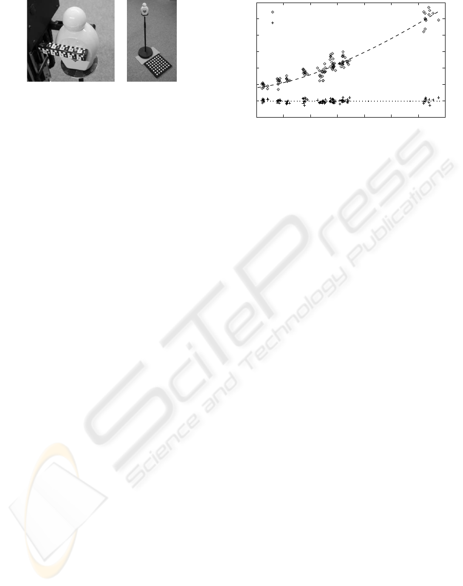
Figure 7: (left) The gripper with the affixed scale, and the
rotational scale on the target. In this example, the grip posi-
tion is 72 mm. (right) The stand with the calibration pattern.
the beginning of each experiment is rather accurate,
only the distance estimation from the robot to the tar-
get is evaluated, and compared to the ground-truth
distance obtained from the calibration pattern.
The final gripping position is determined with the
use of a scale attached to the robot’s gripper (figure
7). The gripping position is defined as the length the
target intrudes into the gripper at the farthest point the
gripper still touches the target. This is compared to
the ideal gripping position of 80 mm.
Figure 8 shows the distance estimation error, plot-
ted against the ground-truth distance (positive values
mean the distance was overestimated; this was the
case in each experiment). Generally, the farther away
the target is, the larger the error in the distance es-
timation becomes. At the same time, the final grip-
ping position, as described above, is not affected by
the starting position. The continuous fusion of new
positional information by the Kalman filter allows the
robot to recover from the inaccurate and uncertain ini-
tial position estimate.
In this application, since the robot moves slowly
enough, the ability to change the zoom level has a
negligible effect on the position estimation, compared
to (for example) the influence of inaccuracies in the
camera vergences. The main benefit of a flexible
zoom level, for this task, occurs during the template
selection scheme. Allowing the template matching to
be performed at higher zoom levels allows one to in-
crease the size of the template in the camera image,
which increases the robustness of the tracking system.
If the robot starts sufficiently far away, using the fixed
minimal zoom level, the template covering the target’s
head is about 16 × 16 pixels. If the zoom level is in-
creased prior to template matching, a larger template
(such as 32 × 32 pixels) can be fitted over the same
target region.
The robot will typically remain at these high zoom
levels at the beginning, gradually reducing the zoom
as it approaches the bottle. This greatly reduces the
chance that the 2D trackers lose the object near the be-
ginning of an experiment; early object loss occurred
in 11 out of 71 experiments with fixed zoom, but only
in 2 out of 62 experiments with a variable zoom, a
reduction of 79%.
−100
0
100
200
300
400
500
600
1400 1600 1800 2000 2200 2400 2600 2800
PSfrag replacements
Initial distance estimation error
Gripping position error
Ground-truth distance (mm)
Error (distance / gripping) (mm)
Figure 8: Evaluation of the distance estimation error and
final gripping position as a function of the ground-truth dis-
tance. As the distance increases, the estimation error in-
creases. However, the gripping position error remains con-
stant. All values are in mm.
To evaluate the object classification, the pose esti-
mate of the target was compared to the ground truth
pose as calculated above to obtain the pose classifi-
cation error. The pose classification error turned out
to be unbiased (near zero mean). The 90th, 75th and
50th percentile of the absolute error is 18.7, 12.5 and
7 degrees, respectively. This compares very favorably
to the cutoff error for acceptance of 20 degrees, as
shown in figure 2(b).
For the evaluation of the grip planning, the pose
estimation from the classifier is added to the action
(movement in degrees) proposed by the grip planner,
for each experiment. This resulting grip angle is com-
pared to the ideal gripping angles (for this target) of
90 and 270 degrees. In our experiments, the plan-
ning error has a mean of -1.52 degrees, with a stan-
dard deviation of 1.36 degrees. This bias is the re-
sult of the cost function applied to the action selection
in section 2.2, as shown in figure 9. Since the target
is equally grippable from two locations, the gripping
system chooses the closer one (requiring less move-
ment) by weighting the action ratings as in equation
(8). A side effect of this weighting is that the modes of
the rating, too, get shifted slightly to favor less move-
ment. This shift, however, is negligible when com-
pared to the pose estimation error.
Finally, the actual gripping angle is evaluated. This
is the pose of the target relative to the robot at step
(5), and is measured externally by use of the scale af-
fixed to the target. This angle is compared to the ideal
gripping angles (90 and 270 degrees in our case) to
obtain the final grip position error. The deviation was
again unbiased (near zero mean), with the 90th, 75th
and 50th percentile at 23, 15 and 9 degrees respec-
tively. As demonstrated in figure 2(b), an absolute er-
ror below 20 degrees was deemed “acceptable”, while
anything above was “not acceptable”. Out of 120 ex-
periments which resulted in grippoint selections, only
ACTIVE SENSING STRATEGIES FOR ROBOTIC PLATFORMS, WITH AN APPLICATION IN VISION-BASED
GRIPPING
175

PSfrag replacements
0
50 100 150 200 250
300 350
10
1
2
3
4
5
6
7
8
9
a
b
Q(s, a)
with costs
no costs
38
◦
Figure 9: Grippoint selection incorporating costs. The tar-
get is estimated to be at 38 degrees. The influence of the
cost function on the rating function is clearly visible.
15 were not acceptable, as the result of an incorrect
pose estimation by the classifier.
4 CONCLUSION AND OUTLOOK
In this paper, we have presented the combination of
two systems, an object tracker and an object classifier,
which are able to grip a non-trivial object using only
visual feedback.
An important aspect is that neither of these systems
require any explicit modeling, neither in the behavior
of the focal length adjustment, nor in the selection of
the gripping angle. Instead, the focal length adjust-
ment comes automatically from the information theo-
retic approach, while the correct angle is trained, al-
lowing the system to generate its own model.
Future work will focus on improving the individ-
ual components of this system, motivated by the goal
of tracking and gripping a moving target. This com-
prises prediction of the target’s position multiple steps
into the future, automatic adaptation of tracking fea-
tures to cope with visually changing objects, and eval-
uation of reinforcement learning techniques which al-
low learning an optimal sequence of actions.
REFERENCES
Bar-Shalom, Y. and Fortmann, T. (1988). Tracking and
Data Association. Academic Press, Boston, San
Diego, New York.
Bertsekas, D. P. (1995). Dynamic Programming and Op-
timal Control. Athena Scientific, Belmont, Mas-
sachusetts. Volumes 1 and 2.
Bicchi, A. and Kumar, V. (2000). Robotic grasping and con-
tact: A review. In Proceedings of the 2000 IEEE In-
ternational Conference on Robotics and Automation,
volume 1, pages 348–353, San Francisco.
Borotschnig, H., Paletta, L., Prantl, M., and Pinz, A. (2000).
Appearance-based active object recognition. Image
and Vision Computing, 18(9):715–727.
Deinzer, F., Denzler, J., and Niemann, H. (2003). Viewpoint
Selection – Planning Optimal Sequences of Views for
Object Recognition. In Computer Analysis of Images
and Patterns – CAIP 2003, LNCS 2756, pages 65–73,
Heidelberg. Springer.
Denzler, J. and Brown, C. (2002). Information Theoretic
Sensor Data Selection for Active Object Recognition
and State Estimation. IEEE Transactions on Pattern
Analysis and Machine Intelligence, 24(2):145–157.
Denzler, J., Zobel, M., and Niemann, H. (2003). Informa-
tion Theoretic Focal Length Selection for Real-Time
Active 3-D Object Tracking. In International Con-
ference on Computer Vision, pages 400–407, Nice,
France. IEEE Computer Society Press.
Grzegorzek, M., Deinzer, F., Reinhold, M., Denzler, J., and
Niemann, H. (2003). How Fusion of Multiple Views
Can Improve Object Recognition in Real-World En-
vironments. In Vision, Modeling, and Visualization
2003, pages 553–560, M
¨
unchen. Aka GmbH, Berlin.
Hager, G. and Belhumeur, P. (1998). Efficient region track-
ing with parametric models of geometry and illumi-
nation. IEEE Transactions on Pattern Analysis and
Machine Intelligence, 20(10):1025–1039.
Mason, M. (2001). Mechanics of Robotic Manipulation.
MIT Press. Intelligent Robotics and Autonomous
Agents Series, ISBN 0-262-13396-2.
Paletta, L. and Pinz, A. (2000). Active Object Recogni-
tion by View Integration and Reinforcement Learning.
Robotics and Autonomous Systems, 31(1–2):71–86.
Puckelsheim, F. (1993). Optimal Design of Experiments.
Wiley Series in Probability and Mathematical Statis-
tics. John Wiley & Sons, New York.
Shannon, C. (1948). A mathematical theory of communi-
cation. The Bell System Technical Journal, 27:379–
423,623–656.
Smith, C. and Papanikolopoulos, N. (1996). Vision-guided
robotic grasping: Issues and experiments. In Proceed-
ings of the 1996 IEEE International Conference on
Robotics and Automation, pages 3203–3208.
Sutton, R. and Barto, A. (1998). Reinforcement Learning.
A Bradford Book, Cambridge, London.
Tordoff, B. and Murray, D. (2001). Reactive Zoom Control
while Tracking Using an Affine Camera. In Proceed-
ings of the 12th British Machine Vision Conference,
volume 1, pages 53–62.
Zobel, M., Denzler, J., and Niemann, H. (2002). Binocu-
lar 3-D Object Tracking with Varying Focal Lengths.
In Proceedings of the IASTED International Confer-
ence on Signal Processing, Pattern Recognition, and
Application, Crete, Greece, pages 325–330, Anaheim,
Calgary, Zurich. ACTA Press.
ICINCO 2004 - ROBOTICS AND AUTOMATION
176