SIMULATION OF SYSTEMS WITH VARIOUS TIME DELAYS

USING PADE'S APPROXIMATION

Mujo Hebibovic, Bakir Lacevic, Jasmin Velagic

Faculty of Electrical Engineering, University of Sarajevo, Zmaja od Bosne bb, 71000 Sarajevo, B&H

Keywords: Time delay, Pade's function, Simulation, Time constant, Taylor series

Abstract: In this paper, Pade's rational functions have been simulated for approximating several characteristic values

of time delay regarding the plant time constant. Several representative plants were tested in order to show in

which cases Pade’s function approximates time-delay block well. Only if the ratio of time delay versus time

constant of the plant is rather great, or the plant contains emphasized numerator dynamics; approximation

capabilities get poorer. The convergence rate of n-order Pade’s function has been also analyzed by using

Taylor series and phase-frequency characteristics.

1 INTRODUCTION

Many of industrial processes and process control

systems, along with their structural presentations,

contain one or more time delay components

(Dugard, Verriest, 1998; Chen, et al., 2003). These

make an inherent part of the mathematical models

used to describe the systems' dynamics of

management and biological systems as well. Padé

approximations are widely used to approximate a

dead-time in continuous control systems (Vajta,

2000). It provides a finite-dimensional rational

approximation of a dead-time. The accuracy of

applied time delay blocks is particularly important in

computer simulation of complex dynamic systems,

described by high-order equations, then in

computation of convolution integrals etc (Beek, et

al., 1999). The principal problem in their realization

is that their transfer function appears in transcendent

form, what is not quite appropriate for simulation

(Hebibovic, 1991; Vajta, 2000). In order to avoid the

problem, it has long been the practice to

approximate the time delay transfer function with a

rational function (Hebibovic, 1998).

In this paper MATLAB/Simulink features were

exploited and comparison of the first four Pade’s

functions has been done regarding several typical

plants and typical ratios of time-delay versus plant

time constant. Convergence that can be seen well

from simulations is supported by theoretical analysis

using Taylor series.

2 SYSTEM DESCRIPTION

Let's consider a time function u(t) as an input of the

time delay block. The output of this system is the

same function, but with time delay τ, which can be

described by Eq.1.

)t(u)t(x

−

(1)

Time delay block can be described in Laplace

form which can be derived from Eq.1.

)s(U

)s(Ue

)s(U

)s(X

)s(G

τ−

=== (2)

Pade's approximation of time delay block is

very favorable in practice because of good

convergence rate of this approximation. It is also

very interesting theoretical case when Pade's

approximation order reaches infinity.

Pade's function is a rational function determined

by Eqs 3-5 (Hebibovic, 1998).

)s(D

)s(N

)s(W

τ−

=τ−

µν

(3)

)s(

)!(!i

)!i(

)s(N τ−

ν+µ

−ν+µ

−ν

=τ−

∑

µν

(4)

)s(

)!(!j

)!j(

)s(D τ

ν+µ

−ν+µ

−µ

=τ−

∑

µν

(5)

289

Hebibovic M., Lacevic B. and Velagic J. (2004).

SIMULATION OF SYSTEMS WITH VARIOUS TIME DELAYS USING PADE’S APPROXIMATION.

In Proceedings of the First International Conference on Informatics in Control, Automation and Robotics, pages 291-295

DOI: 10.5220/0001127402910295

 SciTePress

For practical use, Pade's functon takes form

given by Eq.6 (µ = ν = n)

2n1n0n

sasasaa

sbsbsbb

)s(W

++++

=τ−

(6)

It's obvious that coefficients a

and b

are

functions of time delay τ.

n,,2,1,0i,a)1(b

)!in()!n2(!i

)!in2(!n

K=−=

−

(7)

Number n determines the order of Pade's

function. It can be seen that Pade's coefficients can

be easily arranged into a square matrix. Eqs 8-10

represent some interresting relations between

adjacent members of a matrix. These relations can

simplify software evaluation of Pade's coefficients

(Hebibovic, 1991).

1n,,2,1,0m,

)in2)(1i(

i,n

1i,n

−=τ

−+

−

(8)

()

n,,1,0m,

)1in)(1n2(2

2in2)1in2(

i,n

i,1n

+−+

+−+−

(9)

n,,1,0m,

)1i)(1n2(2

)1in2(

i,n

1i,1n

K=τ

+−

(10)

3 MAGNITUDE AND PHASE OF n-

ORDER PADE'S FUNCTION

Amplitude-frequency characteristic of time delay

block can be perfectly approximated by amplitude-

frequency characteristic of Pade's function. Beside

that, phase-frequency characteristic of Pade's

approximation converges to phase-frequency

characteristic of time delay block, as order of

approximation reaches infinity (Titov, Uspenskij

1969; Doganovskij, Ivanov 1966.)

If ''s'' from Eq.6 gets replaced with ''jω'',

magnitude and phase of observed function can be

easily determined for every number n that represents

order of approximation. All Pade's functions,

represented with Eq.6 have following form

(Hebibovic, 1998).

K,3,2,1n,

jIR

)j(W

nnnn

−

=ωτ−

(11)

It is obvious that magnitude of n-order Pade-s

function is equal to 1 (Eq.12)

K,3,2,1n,1)j(W)(A

nnnn

==ωτ−=ωτ

(12)

Unfortunately, this is not the case for phase-

frequency characteristic (Eqs.13-14)

ωτ−=

ωτ−

)earg(

(13)

ωτ−

≠

−

))j(Warg()(

nnnn

(14)

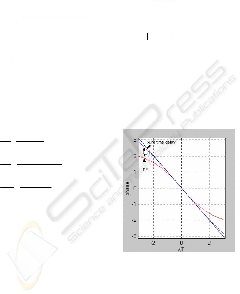
By increasing order of Pade-s function,

equations for phase-frequency characteristic

calculation become more complex, and characteristic

itself converges to phase-frequency characteristic of

pure time delay block (Fig.1, wT ≡ ωτ).

Figure 1: Phase-frequency characteristics of time delay

block and Pade’s functions

The convergence rate of Pade’s function to

transfer function of time delay block can also be

seen from corresponding Taylor series (Eqs 15-17).

ICINCO 2004 - SIGNAL PROCESSING, SYSTEMS MODELING AND CONTROL

290

)e(O

3628800

362880

40320

5040

720

120

s1e

1010

99887766

55443322

τ−

−

+τ−=

(15)

))s(W(O

41472

10368

3456

1728

144

s1)s(W

222

1010

998877

55443322

τ−+

−

+τ−=τ−

(16)

))s(W(O

3628800

362880

40320

5040

720

120

s1)s(W

553

101099

887766

55443322

τ−+

−

+τ−=τ−

(17)

Let k be the number of elements in Taylor’s sum

of W

(-τs), which are identical to corresponding

elements of Taylor’s sum of e

-τs

. Validity of Eq.18

that binds number k with Pade’s function order n can

easlily be shown (Hebibovic, 1998).

1n2

(18)

Hence, if n reaches infinity (n → ∞), than all

corresponding elements of two Taylor’s sums are

identical. Therefore, the next equation can be

written:

)s(Wlime

τ−=

∞→

τ−

(20)

In this case, coefficients of Pade’s polynoms can

be calculated by the following theorem (Hebibovic,

1998).

Theorem: For the order n of Pade’s function

given by the Eq.6 it can be written:

,,2,1,0m,

alima

K=τ==

−

∞→

∞

(21)

Consequences of this theorem are that by

increasing the order of Pade’s function to infinity,

perfect approximation of time delay block by

magnitude and phase is obtained. However, this

approximation can be considered only in domain of

theory. In most practical problems, Pade’s function

with order up to four can satisfy.

4 SIMULATION RESULTS

It is interesting to compare the step response of

block that contains pure time delay to step reponse

of block whose time delay sub-block is

approximated with n-order Pade’s function.

Simulations of plants with various τ/T quotients

have been run, where T represents the time constant

of the process.

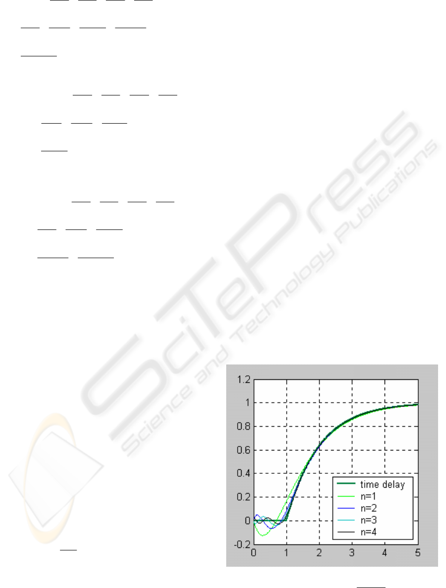
The simulation results are illustrated on Figures 2-9

that presented remarkable feature of Pade’s

approximation. Figures 2-4 show the results

obtained with the first-order static plant including

pure time delay. It is obvious that approximation is

better when τ/T is smaller.

The same procedure has been done with an astatic

first-order plant with several time-delays (Figures 5-

7). The quality of approximation also increases as

τ/T decreases.

Figures 8 and 9 illustrate time responses of

somewhat more complex plant that includes time-

delay. Time response of this transfer function

corresponds to many physiological processes, for

example blood glucose component that is depended

on stress (Hebibovic,

et al., 2003). Empirically, it

can be concluded that the quality of approximation

increases as expression T

T/T

also increases.

Figure 2: Plant

1Ts

e)s(G

τ−

, (τ/T=1)

SIMULATION OF SYSTEMS WITH VARIOUS TIME DELAYS USING PADE'S APPROXIMATION

291

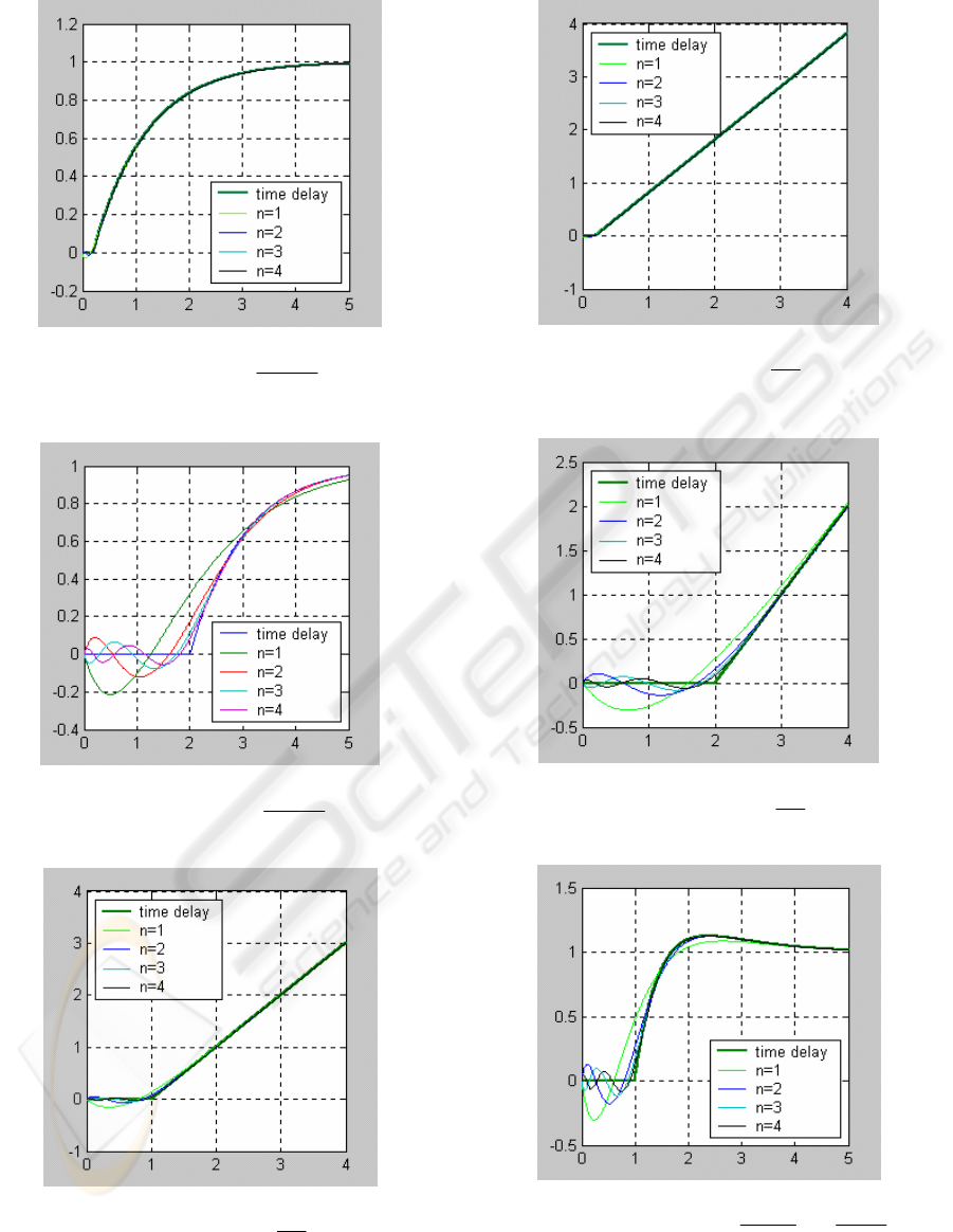
Figure 3: Plant

1Ts

e)s(G

τ−

, (τ/T=0.2)

Figure 4: Plant

1Ts

e)s(G

τ−

, (τ/T=2)

Figure 5: Plant

e)s(G

sτ−

, (τ/T=1)

Figure 6: Plant

e)s(G

sτ−

, (τ/T=0.2)

Figure 7: Plant

e)s(G

sτ−

, (τ/T=2)

Figure 8: Plant

⎟

⎠

⎞

⎜

⎝

⎛

τ−

1Ts

1sT

e)s(G

T/T

≈ τ)

ICINCO 2004 - SIGNAL PROCESSING, SYSTEMS MODELING AND CONTROL

292

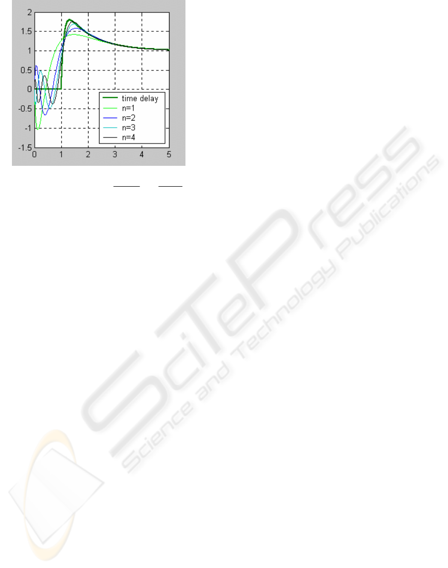
Figure 9: Plant

⎟

⎠

⎞

⎜

⎝

⎛

τ−

1Ts

1sT

e)s(G

T/T

<< τ)

5 CONCLUSIONS

Simulations have shown remarkable features of

Pade's approximation. It can be seen that the time

response of the plant that contains fourth order

Pade's function fits very well the time response of

the plant with pure time delay. This is common for

typical static and astatic industrial processes with

somewhat smaller time delays. However, the quality

of approximation has certain limits. Simulations

show that Pade's approximation doesn't give

satisfactory results for systems with greater time

delays and /or emphasized derivative time constants.

Future work will explore some different models of

rational functions for approximation of time-delay,

especially within the systems where Pade’s function

didn’t show good performance.

REFERENCES

Chen, J., Gu, K., Kharitonov, V. 2003. Stability of Time-

delay Systems, Birkhauser Verlag.

Doganovskij, S.A., Ivanov V.A. 1966. Ustrojstva

zapazdivanija i ih primjenjenie v avtomaticeskih

sistemah, Izdateljstvo Masinostojenie, Moskva.

Dugard, L., Verriest, E.I. 1998. Stability and Control of

Time-delay Systems, Springer-Verlag, Berlin.

Hebibovic, M., 1998. Identification of the block of

transport delay by using Pade’s approximation

(Doctoral dissertation), University of Sarajevo,

Faculty of Electrical Engineering, Sarajevo.

Hebibovic, M., 1991. Fast algorithm for calculating the

coefficients of Pade’s approximation of time delay

block random order, Bilten No 25, Center of RV I

PVO, Rajlovac-Sarajevo.

Hebibovic, M., Lacevic, B., Alagic, S., Kulenovic, I. 2003.

Control of Blood Sugar Components and Their

Computer Aided Modelling, 7th World

Multiconference on Systemics, Cybernetics and

Informatics (SCI 2003), Orlando, USA, July 27-30, pp.

12-16.

Titov, N.I., Uspenskij V.K. 1969. Modelirovanije sistem s

zapazdivanijem, Energija, Leningrad.

Vajta, M. 2000. Some Remarks on Padé-Approximations,

3rd TEMPUS-INTCOM Symposium, September 9-14,

Veszprém, pp. 251-256.

Van Beek, D.A., Rooda, J.E., Trienekens, B.J. 1999.

Hybrid Modelling and Simulation of Time-delay

Elements, In. Proc. of 11th European Simulation

Symposium, Erlangen, pp. 88-92.

SIMULATION OF SYSTEMS WITH VARIOUS TIME DELAYS USING PADE'S APPROXIMATION

293