
ON THE DECENTRALIZED CONTROL OF LARGE
DYNAMICAL COMPLEX SYSTEM
M. Kidouche, M. Zelmat, A. Charef
Faculté des Hydrocarbures et de la Chimie,
Département automatisation et Electrification des Procédés Industriels
Université de Boumerdes 35000, Algéria,
Keywords: Large scale system; decentralized control; singular perturbation approach
Abstract: This paper describes a systematic procedure to build reduced order analytical models for a design
of decentralized controllers for large scale interconnected dynamical systems. The design method
employs Davison techniques to affect decoupling of the interconnections into its subsystems
components which is done by using the most dominant eigenvalues and the most influent inputs
in each subsystem. In this way, advantage can be taken of the special structural feature of a given
system to devise feasible and efficient decentralized strategies for solving large control problem
which are impractical to solve by one shot centralized methods.
1 INTRODUCTION
As many technological environmental or social
systems have a high complexity, large scale systems
became the subject of intensive research in systems
and control theory. The complexity of the system
leads to severe difficulties that are encountered in
the tasks of analyzing the system and designing and
implementing appropriate control strategies
algorithms. These difficulties arise mainly from
dimensionality, uncertainty and information
structure constraints. For these reasons the analysis
and synthesis tasks cannot be solved economically in
a single step as it is possible for similar analysis and
design tasks for small system. Therefore, it is
common procedure in engineering practice to work
with mathematical models that are simpler, but less
accurate, then the best available model of a given
physical process, since the amount of computation
required to analyze and control large scale system
grows faster than its size. It has been long
recognized that it is beneficial to decompose a large
scale system into subsystems, and design control for
each subsystem independently on the basis of the
local subsystems dynamics and the nature of their
interconnections. These are two quite distinct
motivations for this practice:
The first is to reduce the computational burden
associated with simulation, analysis and control
system design.
The second is based on the realization that a
simplified model will lead to simplified control
system design.
2 PROBLEM FORMULATION
Assume the large scale system is given by the
following differential equation
)t(uB)t(xA)t(x
+
=
&
(2.1a)
y(t)= D x(t)
(2.1b)
x(0)=0
(2.1c)
where x is an-vector of states and u is an-vector of
inputs and both A and B are constant matrices of
appropriate dimension, and let us assume that the
system matrix A has distinct eigenvalues. Let the
system described by equation (2.1) be composed of
N subsystems with the i
th
subsystem having x
i
and u
i
as its state and control vectors, respectively. Let the
dimension of x
i
and u
i
be n
i
and m
i
respectively so
that:
∑∑
==
==
N
1i
i
N
1i
i
mmandnn
383
Kidouche M., Zelmat M. and Charef A. (2004).
ON THE DECENTRALIZED CONTROL OF LARGE DYNAMICAL COMPLEX SYSTEM.
In Proceedings of the First International Conference on Informatics in Control, Automation and Robotics, pages 383-389
DOI: 10.5220/0001127203830389
Copyright
c
SciTePress

The global system of (2.1) is assumed to be
completely controllable and global feedback control
law of the form
)t(v)t(xF)t(u +=
(2.2)
has been found using conventional state feedback
control methods so that the eigenvalues of the closed
loop system lie in the pre-assigned location in the s-
plane, where F is an mxn constant matrix, is to be
computed and v is an m-dimensional vector.
The substitution of (2.2) into the system of (2.1)
yields
)t(Bv)t(xA)t(x +=
&
(2.3a)
where
BFAA +=
The decentralized control problem can now be stated
as that of finding a set of decentralized controllers of
the form
)t(v)t(xF)t(u
iiii
+=
(2.4)
where
)nxm(F
iii
In this paper a method is presented for the design of
such controller to the turbine. The design methods
employs appropriate modal and singular perturbation
techniques to affect complete decoupling of the large
scale system into its subsystem components. Once
the decoupling process is complete, the
decentralized controller design problem becomes
that of finding local controllers for each of the
decoupled subsystems in isolation of the rest.
3 EIGENVALUE CONTRIBUTION
MEASURE
For the i
th
subsystem, the n
i
eigenvalues that
contribute most to the controllability of the states of
this subsystem are chosen. Let the similarity
transformation
)t(zM)t(x =
(3.1)
be applied to the open loop system (2.1), where z is
an n-dimensional dummy state vector.
Application of (3.1) to the system of equation (2.1)
gives
)()()( tutzJtz Γ+=
&
(3.2a)
0
1
0
xMz
−
=
(3.2b)
where
)(
1
i
diagAMMJ
λ
==
−
BM
1−
=
Γ
and the system (3.2) experience step changes in all
of its input variable
[
]
T
m21
U)t(u βββ== L
(3.3)
where
k
β
are weighting factors. The steady-state
response of state vectors z is calculated from (3.2) as
ZUJz
ss
=Γ−=
−1
(3.4)
substituting (3.4) into (3.1) gives the following
steady state response
MZx
ss
−
=
(3.5)
In order to determine contribution of the j
th
eigenvalues in the i
th
state variable, the following
measure is used:
jijij
Zm=ω i,j = 1,2,..n
(3.6)
where m
ij
is the element standing on the i
th
row and
j
th
column of the transformation matrix M, and Z
j
is
the j
th
element of the vector Z.
The total contribution of the j
th
eigenvalue,
j
λ
in
σ
states,
σ+++ k2k1k
x,x,x L , is determined from
(3.6) as
∑
σ+
+=
ω=ω
k
1ki
ijj
(3.7)
where k+1 is the index to the σ states.
4 DECOUPLING OF THE
GLOBAL SYSTEM
The decoupling procedure is based on the outcome
of the previous section and on the principals of
singular perturbation techniques. Let the large scale
system (2.1) be written as
)(
)(
)(
)(
)(
2
1
221
121
tu
B
B
tz
tz
AA
AA
tz
tz
x
r
d
r
d
⎥
⎦
⎤
⎢
⎣
⎡
+
⎥
⎦
⎤
⎢
⎣
⎡
⎥
⎦
⎤
⎢
⎣
⎡
=
⎟
⎟
⎠
⎞
⎜
⎜
⎝
⎛
=
&
&
&
4.1)
where
)(tz
d
is (r x 1) aggregated state vector of
subsystem i and
)(tz
r
is (n – r)th order residual
state.
System equations (4.1) can be transformed to its
modal form,
⎥
⎦
⎤
⎢
⎣
⎡
Γ
Γ
+
⎥
⎦
⎤
⎢
⎣
⎡
⎥
⎦
⎤
⎢
⎣
⎡
=
⎥
⎦
⎤
⎢
⎣
⎡
2
1
22
1
2
0
0
v
w
J
J
v
w
&
&
(4.2)
ICINCO 2004 - ROBOTICS AND AUTOMATION
384

.
where w is the vector of retained dominant states
variables,
[]
T
vwMMvx
2
M==
()
AMMJJdiagBlockJ
1
21
−
=−=
[]
BM
T
1
21
−
=ΓΓ=Γ M
and M is a modal matrix. The columns of this matrix
are its eigenvectors, and are ordered in accordance
with the total contribution of each eigenvalue in all
of the states of the ith subsystem
[]
⎥
⎦
⎤
⎢
⎣
⎡
==
221
121
21
MM
MM
M
d
n
dd
µµµ
MLMM
Where
d
i
µ
, i = 1, 2… n are the dominant set of
eigenvectors. Assume that is desired to retain d
()
nd p modes (vector w) of Eq. (4.2), that is
uPwPJPw
T
Γ+=
&
(4.3)
where
[]
0M
d
IP =
(4.4)
and I is an identity matrix of order d partitioned as
the subsystem i; and w = Pv
Let us take the Laplace transform of the lower half
of (4.2) to yield
)()()(
2
1
22
sUJsIsV Γ−=
−
(4.5)
since
2
J represents nondominant modes, Eq. (4.5)
can be approximated by
)()()(
2
1
22
tLutuJtv =Γ−=
−
(4.6)
The partitioned forms of z
r
and v lead to
⎥
⎦
⎤
⎢
⎣
⎡
⎥
⎦
⎤
⎢
⎣
⎡
=
⎥
⎦
⎤
⎢
⎣
⎡
2221
121
v
w
MM
MM
z
z
r
d
(4.7)
2121
vMwMz
d
+=
2221r
vMwMz +=
assuming that M
1
is nonsingular, then by using these
two last equations we get
LuMMMMzMMz
dr
)(
12
1
1212
1
121
−−
++=
uEzNz
dr
+= (4.8)
Eliminating
r
z in Eqs. (4.1)), using Eq. (4.8) leads
to the aggregate decoupled model in condensed form
)t(Hu)t(Gzz
d
+=
&
if we set
)(
~
)( txtz
d
≡ , then
)()(
~
~
tuHtxGx +=
&
NAAG
121
+=
EABH
121
+=
in this method, the effects of the nondominant
modes have been neglected to result in the
decoupled model
5 DECENTRALIZED
CONTROLLER DESIGN
In this section we develop the design of
decentralized controller utilizing the approach
outlined in the previous section.
After identifying the n
i
eigenvalues which make the
largest contribution to the dynamics of the i
th
subsystem, we use the procedure outlined in § 4 to
obtain an approximate model of the i
th
subsystem
given by:
)()(
~
)(
~
tuHtxGtx
iiii
+=
&
i = 1, 2,…N
(5.1)
Thus the overall system can be approximated by
)t(Hu)t(x
~
G)t(x
~
+=
&
(5.2)
where
⎥
⎥
⎥
⎦
⎤
⎢
⎢
⎢
⎣
⎡
=
)t(x
~
)t(x
~
)t(x
~
N
1
M ;
⎥
⎥
⎥
⎦
⎤
⎢
⎢
⎢
⎣
⎡
=
N
1
G0
0G
G
L
MOM
L
;
⎥
⎥
⎥
⎦
⎤
⎢
⎢
⎢
⎣
⎡
=
N
1
H
H
H M
we set
jj
u
β
=
and u
k
= 0, k = 1, 2…m; jk
≠
to
calculate the controllability measure of each of the n
i
eigenvalues of the i
th
subsystem from the j
th
input.
We retain those columns of H
i
that correspond to the
input u
j
that has the largest controllability measure,
which gives the following approximate models of
the i
th
subsystem:
uH
ˆ
)t(x
~
G)t(x
~
iiii
+=
&
(5.3)
where
[]
⎩
⎨
⎧
≠
=
==
kjnull
kjfinite
hH
ˆ
ij
(5.4)
The global approximate model takes the following
form:
)(
ˆ
)()(
~
tuHtGxtx +=
&
(5.5)
where k is the index to those inputs that exert large
influence on the behavior of subsystem i.
Let us assume that the global system described by
(2.1) is completely controllable and a satisfactory
global state feedback control law of the form
vFx)t(u
+
=
(5.6)
ON THE DECENTRALIZED CONTROL OF LARGE DYNAMICAL COMPLEX SYSTEM
385

has been found using existing state feedback control
methods, so that the eigenvalues of the closed loop
system lie in pre-assigned locations in the s-plane.
This gives
)t(Bv)t(xA)t(x +=
&
(5.7)
where
BFAA += is the closed loop system matrix
Next, we design a state feedback controller
vx
~
F
ˆ
u += for the decoupled system (5.5), so that
the closed-loop eigenvalues are the same or close to
those of the original global closed-loop system (5.7).
This yield
vH
ˆ
)t(x
~
G
ˆ
)t(x
~
+=
&
(5.8)
6 EXAMPLE
In this example a four interconnected power system
(TAIPS) will be considered for the application of the
proposed decentralized control approach.
The following state vectors are defined with respect
to [10] as:
)t(Bu)t(Ax)t(x +=
&
where
⎥
⎥
⎥
⎥
⎦
⎤
⎢
⎢
⎢
⎢
⎣
⎡
=
44434241
34333231
24232221
14131211
AAAA
AAAA
AAAA
AAAA
A
such that
Subsystem 1
+
⎥
⎦
⎤
⎢
⎣
⎡
−
+
⎥
⎦
⎤
⎢
⎣
⎡
−−
= )(
6.000
5.04.00
)(
42
00
)(
211
txtxtx
&
)(
1
0
1
tu
⎥
⎦
⎤
⎢
⎣
⎡
=
)()()()(
14143132121
11
tuBxAtxAtxAtxA ++++
where
[][][]
0
1413
== AA
[]
)(01)(
11
txty =
Subsystem 2
)(
6.05.0
04.0
00
)(
5817
100
110
)(
122
txtxtx
⎥
⎥
⎥
⎦
⎤
⎢
⎢
⎢
⎣
⎡
−
−+
⎥
⎥
⎥
⎦
⎤
⎢
⎢
⎢
⎣
⎡
−−−
=
&
+
)(
1
0
0
)(
00
00
03.0
)(
01.0
00
5.00
243
tutxtx
⎥
⎥
⎥
⎦
⎤
⎢
⎢
⎢
⎣
⎡
+
⎥
⎥
⎥
⎦
⎤
⎢
⎢
⎢
⎣
⎡
+
⎥
⎥
⎥
⎦
⎤
⎢
⎢
⎢
⎣
⎡
−
=
)()()()()(
22424323222121
tuBtxAtxAtxAtxA ++++
[]
)(100)(
22
txty =
Subsystem 3
=
⎥
⎦
⎤
⎢
⎣
⎡
+
⎥
⎦
⎤
⎢
⎣
⎡
−
+
⎥
⎦
⎤
⎢
⎣
⎡
−−
=
)(
1
0
)(
005.0
1.000
)(
21
10
)(
3
233
tu
txtxtx
&
)()()()()(
33434131232333
tuBtxAtxAtxAtxA ++
+
+
where
[
]
[
]
[
]
0
3431
=
=
AA
[
]
)(01)(
33
txty
=
Subsystem 4
+
⎥
⎦
⎤
⎢
⎣
⎡
−
+
⎥
⎦
⎤
⎢
⎣
⎡
−−
= )(
000
003.0
)(
209
10
)(
244
txtxtx
&
)(
1
0
4
tu
⎥
⎦
⎤
⎢
⎣
⎡
=
)()()(
44242444
tuBtxAtxA
+
+
;
[
]
0
4341
=
=
AA
[
]
)(01)(
44
txty
=
Following the procedure given in the previous
section we get:
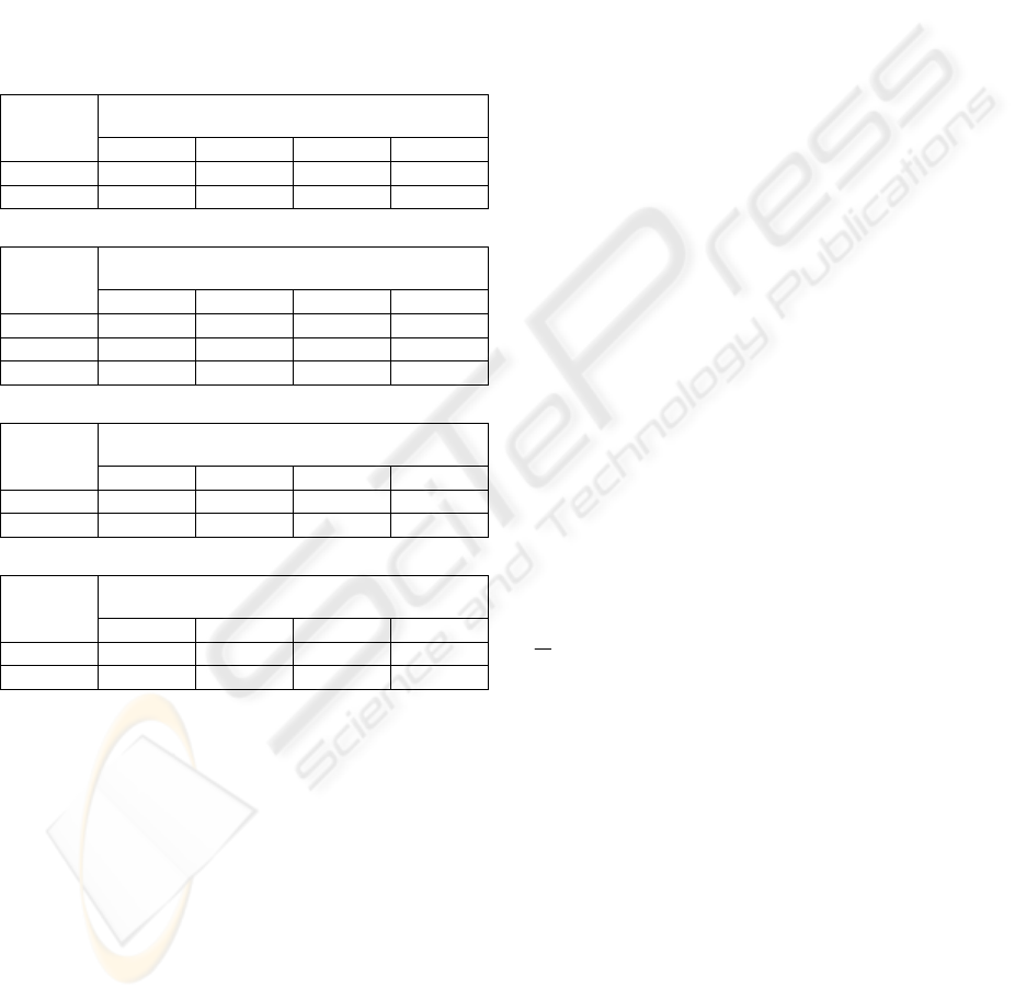
Eigenvalues contributions
Table 1: Eigenvalue contribution measures
X
1,2
X
3,4,5
X
6,7
X
8,9
1
λ
=-19.53
0 0.001 0 0.05
2.405.2
2
j
+
−
=
λ
0.016 0.106 0.004 0.001
2.405.2
3
j
−
−
=
λ
0.016 0.106 0.004 0.001
003.2
4
−
=
λ
0.477 0.115 0.026 0.003
061.0
5
−
=
λ
1.095 0.355 0.018 0.063
01.057.0
6
j
+
−
=
λ
7.897 10.47 4.383 7.153
01.057.0
7
j
−
−
=
λ
7.897 10.47 4.383 7.153
03.006.1
8
j
+
−
=
λ
3.022 30.61 17.98 2.057
03.006.1
9
j
−
−
=
λ
3.022 30.61 17.98 2.057
From the table, we see that
Subsystem 1. The eigenvalues that contribute most
in its states x
1
, x
2
are
7,6
λ
Subsystem 2. The eigenvalues that contribute most
in its states are x
3
, x
4
, x
5
eigenvalues
9,8
λ
Subsystem 3. States are x
6
, x
7
eigevalues
9,8
λ
Subsystem 4. States are x
8
, x
9
eigenvalues
7,6
λ
It is clear from these results that, the relative
contribution measures are satisfactorily high.
ICINCO 2004 - ROBOTICS AND AUTOMATION
386
.
6.1 System decoupling
Application of the decoupling procedure may now
be carried out, incorporating the results of the
previous section. As a result each subsystem is
represented by an approximate model having the
same states as the original subsystem, but with the
input to the global system.
To determine the relative importance of each input
to each subsystem, the controllability measure of the
state of each subsystem from each input must be
evaluated.
Table 2: Controllability measures for subsystem 1
7,6
λ
states
U
1
U
2
U
3
U
4
X
1
0.112 0.268 3.453 0.284
X
2
0.388 0.923 11.89 0.978
Table 3: Controllability measures for subsystem 2
9,8,6
λ
states
U
1
U
2
U
3
U
4
X
1
0.100 0.161 5.256 0.037
X
2
0.476 0.755 25.104 0.095
X
3
0.536 0.850 28.248 0.107
Table 3: Controllability for subsystem 3
9,8
λ
states
U
1
U
2
U
3
U
4
X
1
0.286 0.448 15.271 0.003
X
2
0.357 0.559 19.051 0.004
Table 4: Controllability measures for subsystem 4
7,6
λ
states
U
1
U
2
U
3
U
4
X
1
0.310 0.737 9.499 0.782
X
2
0.143 0.341 4.401 0.362
From the tables, the following conclusion with
regard to the four subsystems can be easily made.
For example; subsystem 1 is most influenced by u
3
,
subsystem 2 is influenced by u
3
and so on.
Accordingly the following approximate
representations for each subsystem are obtained:
)(
37.0
70.0
)(
~
24.132.0
38.109.0
)(
~
311
tutxtx
⎥
⎦
⎤
⎢
⎣
⎡
+
⎥
⎦
⎤
⎢
⎣
⎡
−−
=
&
)(
23.0
19.0
41.0
)(
~
71.18.540250
0209
00.038.4352.19
)(
~
322
tutxtx
⎥
⎥
⎥
⎦
⎤
⎢
⎢
⎢
⎣
⎡
−
+
⎥
⎥
⎥
⎦
⎤
⎢
⎢
⎢
⎣
⎡
−−−
−−=
&
)(
30.0
41.0
)(
~
209
84.3987.17
)(
~
333
tutxtx
⎥
⎦
⎤
⎢
⎣
⎡
−
−
+
⎥
⎦
⎤
⎢
⎣
⎡
−−
=
&
)(
37.0
70.0
)(
~
24.132.0
38.109.0
)(
~
344
tutxtx
⎥
⎦
⎤
⎢
⎣
⎡
−
+
⎥
⎦
⎤
⎢
⎣
⎡
−−
=
&
6.2 Design of optimal controller
The optimal control problem may be stated as that of
finding the control input u(t) which, subject to the
constraints given by the system dynamical
equations, minimizes the following cost function:
[]
dttRututQxtxJ
TT
∫
∞
+=
0
)()()()'
where Q and R are the state and control weighting
matrices, respectively. The solution to this is given
by
u(t) = F x(t) where F is the state feedback optimal
control matrix. If Q and R are chosen as:
Q = diag(0,2,2,0,0,0,2,0,2) and R = (1,16,4,1) then
⎢
⎢
⎢
⎢
⎣
⎡
−
−−
−−
−−
=
0058.0156.0042.0
001.0035.0006.0103.0
001.0001.00002.001.0
03.009.023.044.065.0
F
⎥
⎥
⎥
⎥
⎦
⎤
−−
−
−
0551.0104.00078.0
0003.0129.0001.0
0001.000
0018.0024.00
B
FAA
+
=
have the following set of
eigenvalues:
56.1;23.405.2;48.19
43,21
−=
±
−
=
−
=
λ
λ
λ
j
54.0;301.098.0;05.0
87,65
−=
±
−
=
−
=
λ
λ
λ
j
63.0
9
−
=
λ
⎢
⎢
⎢
⎢
⎣
⎡
−−
−
=
00000
00000
008.072.1838.000
000275.0123.0
~
F
⎥
⎥
⎥
⎥
⎦
⎤
−
−−
275.0123.000
00448.0237.0
0000
0000
ON THE DECENTRALIZED CONTROL OF LARGE DYNAMICAL COMPLEX SYSTEM
387
F
B
A
A
~
~
+= has the following set of eigenvalues
27.2;53.409.2;82.19
43,21
−=
±
−=−=
λ
λ
λ
j
81.0;07.054.0;75.1
87,65
−=
±
−=−=
λ
λ
λ
j
063.0
9
−=
λ
These eigenvalues are close to those of the closed-
loop matrix
A
.
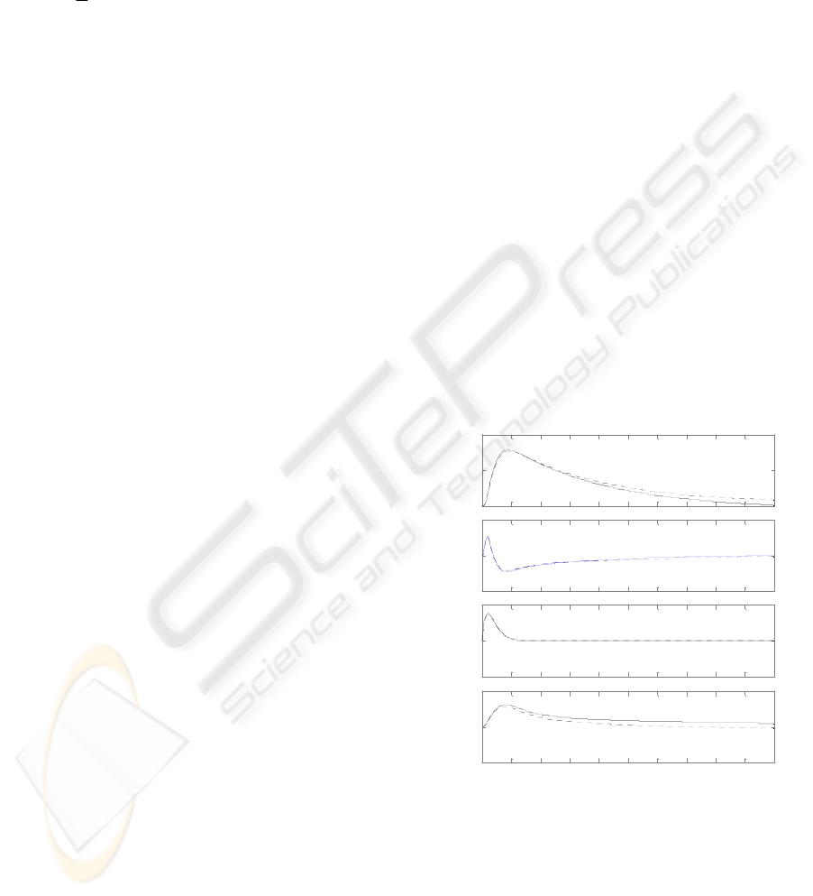
7 SIMULATION RESULTS
Extensive simulation studies on the four subsystem
interconnection have been carried out under both the
decentralized and global optimal controllers. To test
the effectiveness of the decentralized controller, the
closed loop system performance was tested when
multiple changes in the reference settings at different
time intervals were introduced. Figures 1-4 show the
two set of responses overlaid on each other.
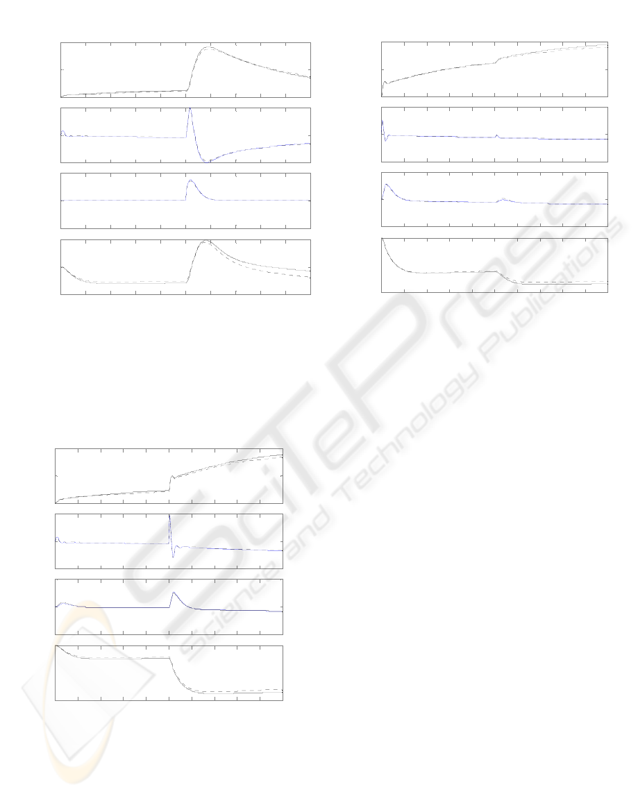
8 CONCLUSION
An interconnected dynamical system comprising
four subsystems has been considered as a study case.
Based on the example studied the proposed design
method appears to be quite attractive. A satisfactory
global optimal controller was designed for the
system. It was shown that the performance of the
decentralized controller designed by using the
method presented is satisfactorily close to that of the
global optimal one.
REFERENCES
M. Kidouche” Overlapping decentralized optimal control
of large scale system” IEEE Int. Conf. on Methods and
Models in Automation and Robotics, 2-5 sept. 2002,
Poland.
J.C. Geromel et al.”Optimal decentralized control of
dynamic systems” Automatica vol.18, N° 5, pp 545-
557, 1982
M. Aldeen and al. “Decentralized PI design method for
interconnected power systems” IEE Proceedings-C
vol.138 N°4 July, 1991
E.J. Davison “The optimal decentralized control of large
scale system: load and frequency control” IEEE
Transactions on automatic control, vol. AC-23, N°2,
April 1978
V.R. Saskino “Singular perturbations and time scale
methods in control theory: survey” Automatica 20, pp
1976-1983; 1984
M. Aldeen and al. “Combined modal and singular
perturbation approach to decentralized control” Int. J.
Systems Sci. vol. 23, N°5, 1992
G.P. Syrcos “Singular perturbation modelling of
continuous and discrete physical systems” Int. J.
Control 37, 1983
M. Kamoun “ Decentralisation de schemas de commande
auto-ajustable de processus de grande dimension »
Rairo, vol.31 pp 289-306, 1997
D.D Siljak « Decentralized control of complex systems »
California Academic Press, 1991
D.D. Siljak “Decentralized control and computations:
Status and prospects: IFAC symposium on large scale
systems: Theory and application, London UK. 10-13
July, 1995
M. Jamshidi “Large scale systems: Modelling and
control » North Holland, New-York, 1983
P.V. Kokotovic “Singular perturbation and iterative
separation of times scales” Automatica 16 (1980) 23.
L. Bakule “Decentralized design of feedback control for
large scale system” Kybernetika, Academia Preha
1988
O. Elgerd “Optimum megawatt-frequency control of
multi-area electric energy system” IEEE Trans. On
Power Apparatus and System, 89, p. 564, 1970
Time (sec. )
A m plitu de
Linear Simulation Results
0
0.1
0.2
To: Y(1)
-0.2
0
0.2
To: Y(2)
-0.5
0
0.5
To: Y(3)
0 5 10 15 20 25 30 35 40 45 50
-0.05
0
0.05
To: Y(4)
Figure 1: Responses to a step change in
3
υ
at t = 0
ICINCO 2004 - ROBOTICS AND AUTOMATION
388
.
Time (sec. )
Am plitude
Linear Simulation Results
0
0.1
0.2
To: Y(1)
-0.1
0
0.1
To: Y(2)
-0.5
0
0.5
To: Y(3)
0 5 10 15 20 25 30 35 40 45 50
-0.02
0
0.02
To: Y(4)
Figure 2: Responses to a step change in
1
υ
at t = 0;
3
υ
at
t = 25s
Time (s ec.)
A m plitu de
Linear Simulation Results
0
0.05
0.1
To: Y(1)
-0.1
0
0.1
To: Y(2)
-0.02
0
0.02
To: Y(3)
0 5 10 15 20 25 30 35 40 45 50
-0.05
0
To: Y(4)
Figure 3: Responses to a step change in
1
υ
at t = 0;
2
υ
at
t = 25s
Time (sec.)
A m plitu d e
Linear Simulation Results
0
0.05
0.1
To: Y(1)
-0.2
0
0.2
To: Y(2)
-0.02
0
0.02
To: Y(3)
0 5 10 15 20 25 30 35 40 45 50
-0.05
0
To: Y(4)
Figure 4: Responses to a step change in
2
υ
at t = 0;
1
υ
at t = 25s
ON THE DECENTRALIZED CONTROL OF LARGE DYNAMICAL COMPLEX SYSTEM
389
