Sensitivity Analysis in OLAP Databases

Emiel Caron and Hennie Daniels

Department of Management, Tilburg University, Warandelaan 2, Tilburg, The Netherlands

Keywords:

OLAP Databases, Business Analytics, Explanatory Analytics, Sensitivity Analysis, Decision-support Systems.

Abstract:

The theoretical underpinnings under which sensitivity analysis is valid in OLAP databases are dealt with in this

paper. Sensitivity analysis is considered to be the reverse of explanation generation in diagnostic reasoning.

Our exposition differentiates between sensitivity analysis in systems of purely drill-down equation and mixed

systems of equations with also business model equations. It is proven that there is an unique additive drill-

down measure deﬁned on all cubes of the aggregation lattice. This proof is the basis for sensitivity analysis in

OLAP databases, where a change in some base cell in the lattice is propagated to all descendants in its upset.

For sensitivity analysis in mixed systems of equations a matrix notation is presented and the conditions for

solvability are discussed. Due to the fact that such systems are typically overdetermined in OLAP databases,

the implicit function theorem cannot be applied. Therefore, we proposed a method to reduce the number of

equations in the system and apply the implicit function theorem on a subsystem of the original system. We

conclude with an alternative method for what-if analysis in mixed systems of equations.

1 INTRODUCTION

The main goal of our research is “to extend the func-

tionality of multi-dimensional (or OLAP) business

databases with diagnostic capabilities to support man-

agerial decision-making” (Caron, 2013). In this pa-

per, the OLAP database is extended with function-

ality for sensitivity analysis. The purpose of the

methods and algorithms presented here, is to provide

OLAP databases with more powerful explanatory an-

alytics and reporting functions. In this paper, we de-

scribe how sensitivity analysis can be implemented in

a multi-dimensional database.

Sensitivity analysis in multi-dimensional

databases is related to the notion of comparative

statics in economics. Where the central issue is to

determine how changes in independent variables

affect dependent variables in an economic model.

Comparative statics is deﬁned as the comparison of

two different equilibrium states solutions, before and

after a change in one of the independent variables,

keeping the other variables unchanged (Samuelson,

1941). It is one of the primary analytical methods

used in economics, where it is commonly used, for

example, in the study of changes in supply and de-

mand when analyzing a market. Instead of repeating

the phrase “keeping the other variables unchanged”,

economists use the more compact Latin equivalent

ceteris paribus (c.p.). The underlying model for

comparative statics is a set of equations that deﬁne

the vector of dependent variables y

,...,y

functions of the vector of independent variables

,...,x

, i.e.

y = f

(x),l = 1,2,...,m. (1)

On the one hand, this corresponds to a system of busi-

ness model equations between measures in an OLAP

database. Relations between measures are denoted by

(C)), (2)

where y and x = (x

,...,x

) are measures on the

same cube C = [i

,...,i

]. On the other , the ap-

plication of a speciﬁc aggregation function f , i.e.

SUM(), Count(), AVG(), etc., on the measure values

of each cube y(C) in L creates a system of drill-down

equations, given by

...i

...(i

−1)...i

−1

(C))). (3)

In Equation (2), the function f might be non-

linear, in Equation (3), the function f is linear for

SUM() and Count() aggregations, where R is a drill-

down operator in dimension q. In the latter situa-

tion we use the terms non-base variables and base

variables, for dependent and independent variables,

respectively. To implement sensitivity analysis in

OLAP, we deﬁne a new cube operator that supports

Caron, E. and Daniels, H.

Sensitivity Analysis in OLAP Databases.

DOI: 10.5220/0006791702210228

In Proceedings of the 20th International Conference on Enterprise Information Systems (ICEIS 2018), pages 221-228

ISBN: 978-989-758-298-1

221

the analyst in answering typical managerial what-if

questions, while navigating the cube. We distinguish

between two types of what-if questions:

• Questions related to a system of drill-down equa-

tions. For example, “How is the proﬁt in the year

2010 affected when the proﬁt for a certain product

is changed with one percent in the ﬁrst quarter in

The Netherlands, c.p.?”

• Questions related to a system of business model

equations. For example, “How is the proﬁt in the

year 2010 for a certain product affected when its

unit price is changed with one additional unit in

the sales model, c.p.?”

This paper is structured as follows. In Subsection

1.1 we discuss related work. In Section 2 we discuss

sensitivity analysis in systems that consist of purely

drill-down equations. In Section 3 we elaborate on

sensitivity analysis in systems that consist of purely

business model equations and mixed systems of equa-

tions. Finally, in Section 4 we draw some conclu-

sions.

1.1 Related Work

The variables, parameter values, and assumptions

of any business or economic model are subject to

change. Sensitivity analysis, generally deﬁned, is

the investigation of these potential changes and their

impacts on conclusions to be drawn from the model

(e.g. (Baird, 1990)). There are many possible appli-

cations of sensitivity analysis, described here within

the categories of decision support, communication,

increased understanding or quantiﬁcation of the sys-

tem, and model development (Pannell, 1997). There

is a very large literature on procedures and techniques

for sensitivity analysis (Clemson et al., 1995). Two

general classes of techniques for sensitivity analy-

sis are the implicit function theorem (Currier, 2000;

Heckman, 2000) and monotone comparative statics

(Milgrom and Shannon, 1994). These are methods

for characterizing whether an increase in a parame-

ter causes the dependent variable to increase or de-

crease. Historically the implicit function theorem was

used for this purpose and the implicit function theo-

rem not only tells you whether the dependent vari-

able increases or decreases but also the magnitude of

change. In contrast, monotone comparative statics

tells you only “up” or “down”, i.e., it gives an ordi-

nal rather than cardinal answer. In our research, we

focused solely on quantitative what-if analysis within

the multi-dimensional database.

To the best of our knowledge, (Balmin et al.,

2000) and (Lakshmanan et al., 2007) are the only pub-

lished research works that address sensitivity analysis

in OLAP databases in a signiﬁcant way. In (Balmin

et al., 2000), the authors have developed the SESAME

system for the processing of hypothetical queries. For

this system query algebra operators are proposed that

are suitable for spreadsheet-style what-if computa-

tions. In the system hypothetical queries are mod-

eled as a list of hypothetical modiﬁcations on the data

in the fact table. A shortcoming of their approach is

that it lacks a good mathematical underpinning, to de-

cide whether a certain change is allowed in the model

or not, as opposed to our approach. In (Lakshmanan

et al., 2007), a different perspective is taken on what-

if analysis. They focus on what-if analysis related to

changes in dimensions and their hierarchical struc-

ture. However, our focus is on data-driven what-if

scenarios, as opposed to structural ones.

In many OLAP software products, sensitivity

analysis is not possible at the moment. If one wants

to do sensitivity analysis in these products one has

to copy the data to a reporting environment, for ex-

ample MS Excel, to compute manually the impact of

changes in certain cells of the data cube. An excep-

tion is the software product Clickview (Cliqview Cor-

poration, 2017), where a ﬁxed change in a base vari-

able can be induced in a system of additive drill-down

measures, to determine its impact on non-base vari-

ables. The difference with our approach is that we can

induce variable changes in systems of additive and av-

erage drill-down measures and under certain condi-

tions in non-linear systems of business equations. For

this purpose we have designed a prototype application

for sensitivity analysis in MS Excel with Pivot tables,

with additional features implemented in Visual Basic.

2 SENSITIVITY ANALYSIS IN A

SYSTEM OF DRILL-DOWN

EQUATIONS

In this section we investigate the inﬂuence of a change

in a measure value of a cell in any OLAP cube, on a

higher level value of the same measure in the aggrega-

tion lattice. Or in formal notation, what is the effect

of changing y(c

) to y(c

) + δ on a dependent vari-

able y(c) in the upset of c

. To solve this consider the

lattice L

with top cube C

= [i

,...,i

] and base

cube C

= [ j

, j

,..., j

]. Notice that L

is a sublat-

tice of L and L

= {↓ c} ∩ {↑ c

}. The values of the

measure y in the cube C

are denoted by x(c

), and

are called the base variables where i = 1,2,...,|C

and the values of the measure y in {↑ C

} are de-

noted by y(c), and are called the non-base variables.

We distinguish between the original values of a mea-

ICEIS 2018 - 20th International Conference on Enterprise Information Systems

222

sure without change x

) and y

), and the values

of the changed measure: x

) and y

), where

) = x

) except for one cell c

in the cube C

for which x

) − x

) = δ.

The following theorem shows how the values of y

change in the lattice L

Theorem 1. There is an unique additive drill-

down measure y

sublattice L

such that:

) − x

)), (4)

where:

β(c) = 1 if c ∈ {↑ c

}, and

β(c) = 0 if c /∈ {↑ c

Proof. To show that y

show that β(c) · (x

) − x

)) is additive, because

the sum of additive measures is also additive and y

(c)

is additive by the consistency assumption. Hence, we

must show that:

β(c) =

∑

β(R

−1

(c)), (5)

where R

−1

is the drill-down operation deﬁned on a

cell c in the lattice L. Now there are two cases:

1. c ∈ {↑ c

}, i.e. c is an ancestor of c

. In that case c

is also a descendant of one of the cells in R

−1

(c),

∈ {↓ R

−1

(c)}, which is a child of c in dimension

q. This property does not depend on dimension q.

So both sides of Equation (5) are equal to 1.

2. c /∈ {↑ c

}, i.e. c is not an ancestor of c

. In that

case, c

is also not a descendant of one of the chil-

dren of c. Hence, both sides of Equation (5) are

zero. 

Notice that the drill-down measure y

unique. This follows from the general proposition that

every additive measure with given values on the base

cube is unique. This follows immediately from The-

orem on OLAP equations described in (Caron, 2013)

(page 40), and the fact that L

is a lattice of cubes.

In the case that c ∈ {↑ c

}, we can rewrite Equation

(4) as follows

),y

(c)). (6)

If y(c) is an additive drill-down measure then we use

inf(y

a;j

),y

a;i

(c)) = y

a;j

) − y

r;j

), (7)

for the computation of inf(y

),y

(c)) in Equa-

tion (6) and if the variable x

) is changed with

δ in sensitivity analysis then y

) − x

)). This result follows

immediately from the Theorem described in (Caron,

2013) (page 40).

Moreover, in the case that y

down measure we use speciﬁc inﬂuence measure for

the computation of inf(y

),y

(c)) in Equation (6)

and if the variable x

) is changed with δ in sen-

sitivity analysis then y

) − x

)), where C

is the context

cube under consideration. This result is not proven

here but the proof is similar to the proof of Theorem

described in (Caron, 2013) (page 40), with the differ-

ence that the RHS of the drill-down equation is di-

vided by the number of cells in the context cube.

Here we present a numeric example of a what-if

analysis in the cube C = Store × Products for the

measure sales, aggregated by the average function.

The data of the cube is depicted in Table 1. We want

to analyse a change δ in the cell (A,P

) on its upset

{↑ (A,P

)}. The reference value of the cell is given

by sales

(A,P

) = 1 and the actual value is given

by sales

(A,P

) = 1 + δ. By applying Equation (6)

we compute the effect of this change on {↑ (A,P

)};

these effects are given by,

sales

(All,P

) = sales

(All,P

) +

δ where |R

Stores

(C)| = 3,

sales

(A,All) = sales

(A,All)+

δ where |R

Products

(C)| = 4,

sales

(All,All) = sales

(All,All)+

δ where |C| = 12.

For example, here R

Stores

(C), represent a roll-up (+1)

in the Stores’s dimension hierarchy, and |R

Stores

(C)| =

3 represents the number of stores.

Table 1: Sensitivity analysis in the example cube Store ×

Products for the average drill-down measure sales. Here the

value of the cell (A, P

) is changed with δ and this change

is propagated in the cell’s upset.

AVG(sales) Stores

Products

A B C All

1 + δ 2 3 2 +

4 5 6 5

7 8 9 8

10 11 12 11

All 5.5 +

δ 6.5 7.5 6.5 +

The subsystem of drill-down equations that cor-

responds with {↑ c

} has an unique solution, after a

change in y(c

) with some δ, as a result of the theo-

rem (Caron, 2013) . However, the complete system of

equations becomes inconsistent because Equation (3)

does not hold in that case:

max

...max

) 6=

∑

∈R

−max

◦...◦R

−max

◦R

−max

(c)

00...0

In other words, when the change in what-if analysis

is not induced by a variable in the base cube, but by a

Sensitivity Analysis in OLAP Databases

223

(non-base) variable on some intermediate level in the

lattice L, the complete system of equations will be-

come inconsistent. For analysis restricted to {↑ c

}

this does not matter, however analysis in the com-

plete system is obviously not useful anymore. The

inconsistencies in the complete system of drill-down

equations, can be corrected by a straightforward pro-

cedure, that repairs the OLAP database (Caron and

Daniels, 2008).

3 SENSITIVITY ANALYSIS IN A

SYSTEM OF BUSINESS

EQUATIONS

In this section we discuss managerial what-if ques-

tions related to a system of business model equations

and a mixed system of drill-down and business model

equations.

Multiple related measures in the business model

and associated dimensions, result in a mixed, often

non-linear, system of equations. For example, con-

sider Table 2 with the equations of Figure 1. In 13

these equations are given in shorthand notation. The

system of equations in (13) are represented as a graph

in Figure 2. In this system we want to change an in-

dependent variable x

, e.g. x

(= Volume(2005.Q2))

and/or x

(= Unit Price(2005.Q2)), and study the im-

pact on its upset, in particular, the dependent root

variable y

(= Revenues(2005)). Notice that (13) is

overdetermined, because we have 4 independent vari-

ables and 5 equations.

In general, for a mixed system of equations

• the equations are linear and non-linear, and

• the system of equations is overdetermined.

Similarly, a system of solely drill-down equations is

also overdetermined in the case of multiple dimen-

sions. Equation (13) can be written as

(y,x) = 0. (8)

The linearization of (8) in a neighborhood of a solu-

tion (y

) reads:

y + A

x = 0. (9)

The matrix A

is the l × m coefﬁcient submatrix for

dependent variables and A

is the l ×n coefﬁcient sub-

matrix for independent variables. Here the matrix of

the ﬁrst derivatives of f with respect to y is represented

by A

= D

f(y,x) and the matrix of ﬁrst derivatives of

f with respect to x is represented by A

= D

f(y,x).

With (9) we can examine the impact of a change in

one or more independent variables c.p., given by ∆x,

on the dependent variables, given by ∆y, where equa-

tion (8) has to be satisﬁed. In the next section, we in-

vestigate the conditions for consistency and solvabil-

ity of (9), which is a necessary condition for solvabil-

ity of (8).

3.1 Conditions for Solvability

A necessary condition for solvability in a system of

linear equations is the rank criterium. A system of

linear equations (9), of A

y + A

x = 0, is solvable if

and only if rank(A

| − A

x) = rank(A

). The proof of

this theorem is, for example, given in (Schott, 1997).

In words, the rank criterium says that the vector −A

must be in the column space (range) of A

for the sys-

tem to be solvable.

To investigate the solvability of (8), we assume

that

) = (y

,...,y

,...,x

)

is a solution of (8). We substitute this solution in

the derivative matrices A

and A

to obtain the lin-

earized matrix [A

] at the solution (y

). The

linearized system of equations A

∆y + A

∆x = 0 is

solvable if and only if rank(A

) = rank(A

| − A

∆x).

Similarly, the linearized system of equations is solv-

able for an independent variable ∂x

, if and only if,

rank(A

) = rank(A

|column x

from A

). A column

vector x

of the submatrix A

is represented by a

(i).

Accordingly, the rank criterium can be used to deter-

mine whether an independent variable ∂x

qualiﬁes for

what-if analysis in a system of business model equa-

tions. However, in the next section it is shown, that

this criterium is a necessary but not sufﬁcient condi-

tion for the solvability of a non-linear system of equa-

tions.

When the submatrix A

is nonsingular then the so-

lution of A

∆y + A

∆x = 0 is unique and given by

∆y = −A

−1

∆x.

Notice that the rank criterium is a necessary but not

sufﬁcient condition for the solvability of a non-linear

system of equations. Practically, this means that in

such models the number of equations must be equal

to the number of dependent variables to produce a

square submatrix A

(l = m).

Now suppose that we are given an overdetermined

system of equations as in (8) and a solution (y

) to

this system such that all the equations are satisﬁed.

The ﬁrst derivatives of the equations can be written

in matrix form as in (9). If the rank criterium for

consistency holds for a certain independent variable

, considered for what-if analysis, then the solution

f(y

) = 0 is ﬁlled in Equation (9). Subsequently,

· eq. 1 + α

· eq. 2 + . . . + α

· eq. l = 0, (10)

ICEIS 2018 - 20th International Conference on Enterprise Information Systems

224

holds if all the α

’s exist. If the α

’s exist we re-

move (l − m) dependent equations from the system of

equations and derive a (m × m) submatrix A

. If the

remaining system of equations in A

is nonsingular

the implicit function theorem can be applied and the

’s determined. In that case the removed equations

are satisﬁed too, because Equation (10) holds and the

general solution for x

can be determined.

3.2 What-if Analysis Example

In this example we want to change an independent

variable x

and study the impact on elements in its up-

set. The Jacobian of the system of equations in (13)

is given in (14). Observe that the vector

) = (48 16 15 3.2|13 12 7 4 4 6 3 2 2.75 3 3.25),

is a solution to the system of equations. The Ja-

cobian at (x

) is given in (15) The rank cri-

terium for solvability in this system is satisﬁed for

the variables x

(= Volume(2005.Q2)) and x

(= Unit

Price(2005.Q2)): rank(A

2(4)

) = rank(A

) = 4 and

rank(A

2(5)

) =rank(A

) = 4. It can easily be veri-

ﬁed that the rank criterium is not satisﬁed for the other

independent variables. For example, for variable x

it can be concluded that rank(A

2(1)

) > rank(A

Therefore, the only candidate independent variables

for what-if analysis in this example are x

and x

As we saw, the rank criterium is a necessary but

not sufﬁcient condition for solvability. We cannot ap-

ply the implicit function theorem to verify solvability

here, because the submatrix A

is non-square (5 × 4).

But in this case we may eliminate one of the equations

because we can ﬁnd α

such that:

· eq. 1 + α

· eq. 2 + α

· eq. 3+

· eq. 4 + α

· eq. 5 = 0.

(11)

These α

’s are given by



















−1







Now we proceed as follows. In the system of equa-

tions in (13) all independent variables are replaced

by the solution (y

) except the independent vari-

ables x

and x

, that are under consideration for what-

if analysis. From the original system of equations,

one dependent equation is removed and we derive a

reduced system of equations, where the matrix A

square. Removing eq. 2 yields

f (y

) =











−y

+ 32 + y

= 0

−y

+ x

= 0

−y

+ 11 + x

= 0

−y

+ (32 + x

)/y

= 0.

(12)

) = (48,16,15,3.2,4,4) is a solution of (12).

The 4 × 4 derivative submatrix A

of f with respect to

y in (48, 16, 15, 3.2, 4, 4) is

f(48,16,15,3.2,4,4) =







−1 1 0 0

0 −1 0 0

0 0 −1 0

0 0 −

225

−1







= A

It can easily be veriﬁed that

−1







−1 1 0 0

0 −1 0 0

0 0 −1 0

0 0 −

225

−1













−1 −1 0 0

0 −1 0 0

0 0 −1 0

0 0

225

−1







= I

By the implicit function theorem we can ﬁnd con-

tinuous differentiable functions ϕ

) : B → R,

where B = B

(48,16,15,3.2,4,4), such that











= ϕ

)

= ϕ

)

= ϕ

)

= ϕ

is a solution of the system of equations (12). More-

over, also the removed equation −y

+ y

= 0 (eq.

2) is satisﬁed because of (11). Computation gives:











= 32 + x

= (11 + x

)(

32+x

11+x

) = 32 + x

= x

= 11 + x

32+x

11+x

4 CONCLUSIONS

In this paper, we stated the theoretical underpinnings

under which sensitivity analysis is allowed in multi-

dimensional databases. We also discussed some the-

oretical issues and procedures related to sensitivity

analysis in OLAP databases.

For sensitivity analysis in systems of additive

drill-down measures we proved Theorem 1, and

Sensitivity Analysis in OLAP Databases

225

showed that there is an unique additive drill-down

measure y

lattice. This theorem is the basis for sensitivity analy-

sis here, where a change in some base cell in the lat-

tice is propagated to all descendants in its upset. For

the average drill-down measure a similar expression

is determined. Moreover, sensitivity analysis might

cause the multi-dimensional database to become cor-

rupted, if the analysis is not carried out on cells in the

base cube. To overcome this problem we proposed a

correction procedure.

For sensitivity analysis in mixed systems of equa-

tions we introduced a matrix notation and we dis-

cussed the conditions for solvability. Because mixed

systems are typically overdetermined the implicit

function theorem cannot be applied. Therefore, we

proposed a method to reduce the number of equations

in the system and apply the implicit function theorem

on a subsystem.

REFERENCES

Baird, B. (1990). Managerial Decisions Under Uncer-

tainty: An Introduction to the Analysis of Decision

Making. John Wiley & Sons, Inc., New York.

Balmin, A., Papakonstantinou, Y., and Papadimitriou, T.

(2000). Optimization of hypothetical queries in an

olap environment. Data Engineering, International

Conference on, 0:311.

Caron, E. (2013). Explanation of Exceptional Values in

Multi-dimensional Business Databases. PhD thesis,

Erasmus University.

Caron, E. A. M. and Daniels, H. A. M. (2008). Ex-

tensions to the olap framework for business analy-

sis. In Cordeiro, J., Shishkov, B., Ranchordas, A.,

and Helfert, M., editors, ICSOFT (ISDM/ABF), pages

240–247. INSTICC Press.

Clemson, B., Yongming, T., Pyne, J., and Unal, R. (1995).

Efﬁcient methods for sensitivity analysis. System Dy-

namics Review, 11(1):31–49.

Cliqview Corporation (2017). Cliqview.

Currier, K. (2000). Comparative Statics Analysis in Eco-

nomics. World Scientiﬁc Publishing Co, Singapore.

Heckman, J. (2000). Causal parameters and policy analysis

in economics: A twentieth century retrospective. The

Quarterly Journal of Economics, 115(1):45–97.

IBM Cognos Software (2017). Ibm cognos business intelli-

gence, powerplay.

Lakshmanan, L., Russakovsky, A., and Sashikanth, V.

(2007). What if olap queries with changing dimen-

sions perspectives are everything. In VLDB ’07: Pro-

ceedings of the 33th International Conference on Very

Large Data Bases, San Francisco, CA, USA. Morgan

Kaufmann Publishers Inc.

Milgrom, P. and Shannon, C. (1994). Monotone compara-

tive statics. Econometrica, 62(1):157–80.

Pannell, D. J. (1997). Sensitivity analysis of normative eco-

nomic models: theoretical framework and practical

strategies. Agricultural Economics, 16(2):139–152.

Samuelson, P. A. (1941). The stability of equilibrium:

Comparative statics and dynamics. Econometrica,

9(2):97–120.

Schott, J. (1997). Matrix Analysis for Statistics. Wiley, New

York.

ICEIS 2018 - 20th International Conference on Enterprise Information Systems

226

APPENDIX

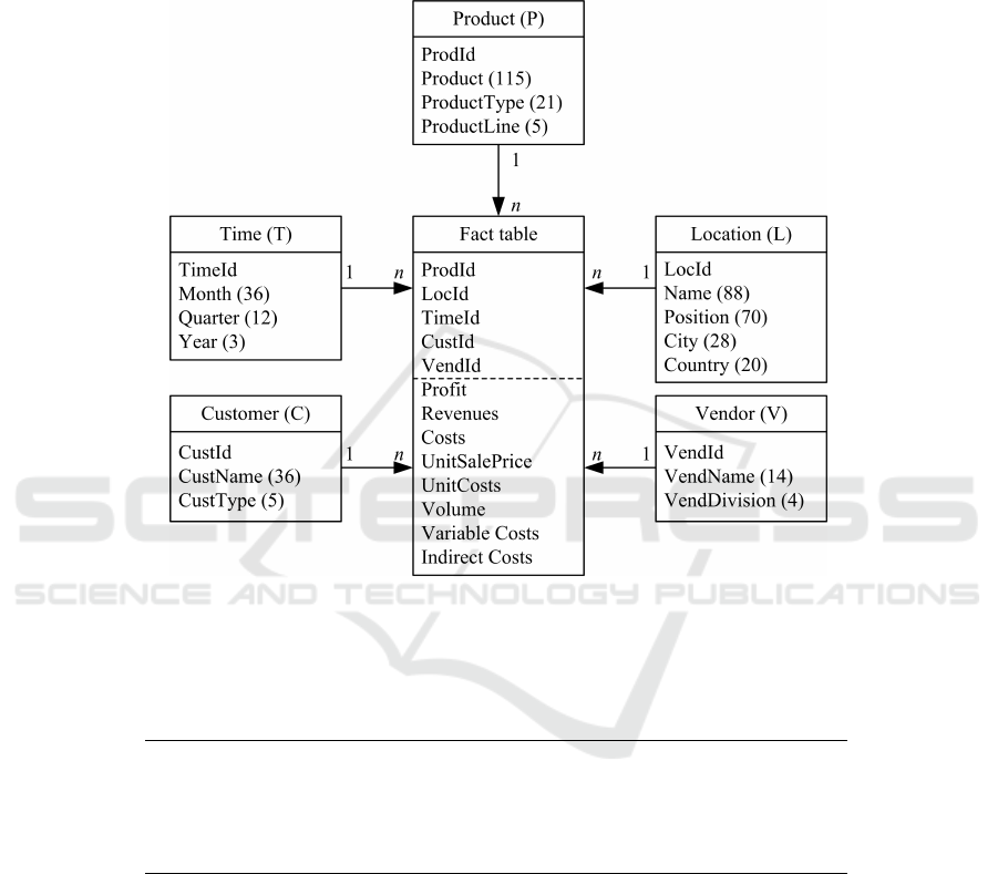
A star model representing a multi-dimensional ﬁnancial database is shown in Figure 1 and is used as an illustra-

tive example in this paper. This database, called GoSales, contains the ﬁnancial ﬁgures from a generic ﬁctitious

company that sells sports equipment, obtained from the Cognos OLAP product PowerPlay (IBM Cognos Soft-

ware, 2017). Figure 1 depicts a central fact table and ﬁve dimensions tables. The central fact table represents the

Figure 1: Star model with ﬁve dimension tables and a central fact table representing the ﬁnancial data set.

ﬁnancial data set. It lists the measures of the data, like proﬁt, revenues, costs, etc. The ﬁnancial data set has ﬁve

dimensions tables: Time (T), Product (P), Location (L), Customer (C), and Vendor (V), and all dimensions have

a 2-4 level hierarchy.

Table 2: Subsystem of business model and drill-down equations derived from a multi-dimensional ﬁnancial database.

1. Rev.(2005) = Rev.(2005.Q1) + Rev.(2005.Q2) + Rev.(2005.Q3) + Rev.(2005.Q4)

2. Rev.(2005) = Vol.(2005) × Unit Pr.(2005)

3. Rev.(2005.Q2) = Vol.(2005.Q2) × Unit Pr.(2005.Q2)

4. Vol.(2005) = Vol.(2005.Q1) + Vol.(2005.Q2) + Vol.(2005.Q3) + Vol.(2005.Q4)

5. Unit Pr.(2005) = ((Vol.(*.Q1) × Unit Pr.(*.Q1)) + (Vol.(*.Q2) × Unit Pr.(*.Q2)) +

(Vol.(*.Q3) × Unit Pr.(*.Q3)) + (Vol.(*.Q4) × Unit Pr.(*.Q4))) / Unit Pr.(*)

Table 2 in shorthand notation











−y

+ x

+ y

+ x

= 0

−y

+ y

× y

= 0

−y

+ x

× x

= 0

−y

+ x

= 0

−y

+ ((x

× x

) + (x

× x

) + (x

× x

) + (x

× x

))/y

= 0,

(13)

where y

with i = 1, 2, 3, 4 are the dependent variables and x

with i = 1, 2, . . . , 11 are the independent variables.

Sensitivity Analysis in OLAP Databases

227

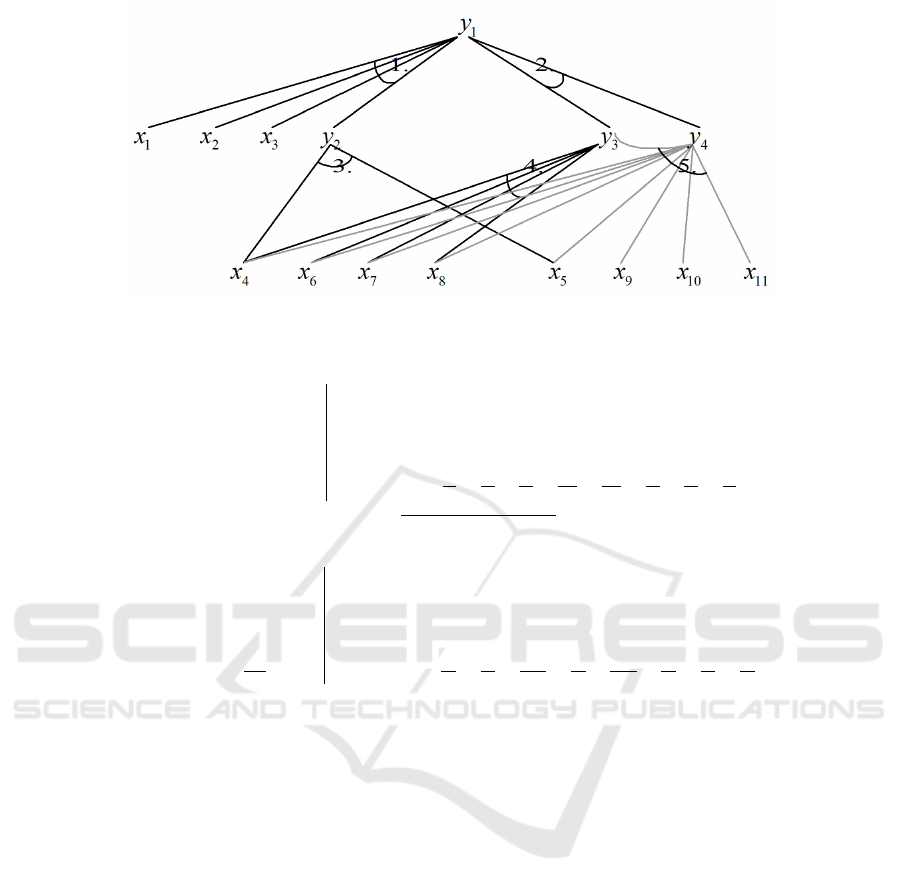
Figure 2: Graph representation of the implicit system of equations.

A = [A

] =







−1 1 0 0 1 1 1 0 0 0 0 0 0 0 0

−1 0 y

0 0 0 0 0 0 0 0 0 0 0

0 −1 0 0 0 0 0 x

0 0 0 0 0 0

0 0 −1 0 0 0 0 1 0 1 1 1 0 0 0

0 0 )

∗

−1 0 0 0







)

∗

= −

)

(14)

= [A

] =







−1 1 0 0 1 1 1 0 0 0 0 0 0 0 0

−1 0 3.2 15 0 0 0 0 0 0 0 0 0 0 0

0 −1 0 0 0 0 0 4 4 0 0 0 0 0 0

0 0 −1 0 0 0 0 1 0 1 1 1 0 0 0

0 0 −

225

−1 0 0 0

2.75

3.25







(15)

ICEIS 2018 - 20th International Conference on Enterprise Information Systems

228