Error Correction over Optical Transmission
Weam M. Binjumah
1,2
, Alexey Redyuk
3
, Rod Adams
1
, Neil Davey
1
and Yi Sun
1
1
The School of Computer Science, University of Hertfordshire, Hatfield, U.K.
2
The Community College, Taibah University, Madinah, Kingdom of Saudi Arabia
3
Institute of Computational Technologies SB RAS, Novosibirsk, Russia
Keywords:
Support Vector Machine (SVM), Machine Learning, Optical Signals, Coherent Optical Communications,
Error Correction, Wavelet Transform.
Abstract:
Reducing bit error rate and improving performance of modern coherent optical communication system is a
significant issue. As the distance travelled by the information signal increases, bit error rate will degrade.
Support Vector Machines are the most up to date machine learning method for error correction in optical
transmission systems. Wavelet transform has been a popular method to signals processing. In this study, the
properties of most used Haar and Daubechies wavelets are implemented for signals correction. Our results
show that the bit error rate can be improved by using classification based on wavelet transforms (WT) and
support vector machine (SVM).
1 INTRODUCTION
Improving the bit error rate (the number of bit errors
divided by the total number of transmitted bits) in op-
tical transmission systems is a crucial and challeng-
ing problem. There are many different causes of the
transmitted signal degradation in optical communica-
tion systems, for instance optical losses, fiber nonlin-
earity, dispersive properties of the medium etc (Bern-
stein et al., 2003). Increasing the distance travelled
by the optical pulses along long-haul fiber links also
leads to an increase in the number of error bits. In op-
tical telecommunications an information signal may
be encoded by amplitude or the phase of the optical
pulses. In this work, we consider phase encoding sig-
nals. Metaxas et al. demonstrates that linear Support
Vector Machines (SVM) outperformed other trainable
classifiers, such as using neural networks, for error
correction in optical data transmission; besides that it
is easier to build the hardware for an SVM in real time
(Metaxas et al., 2013).
The purpose of signal decomposition is to extract
the relevant information from the signal and reduce
the level of interfering noise. The wavelet transform
has become widespread in analyzing and processing
signals. Wavelet signal processing can be applied to
extract the underlying information of the signal (Ri-
oul and Vetterli, 1991). For various kinds of signals,
different kinds of wavelets can be selected. In this pa-
per, we investigate whether wavelets can be used on
the distorted optical signals to extract the reliable in-
formation of the original signals or not. Especially,
we look into whether wavelets can deal with noise in
phase and/or frequency of optical signals.
2 PROBLEM DOMAIN
Typical optical communication systems consist of
three main components, see Figure 1: an optical trans-
mitter (Tx in Figure 1) that converts the electrical sig-
nal into an optical signal, an optical fiber as the prop-
agation medium of the optical signal and an optical
receiver (Rx in Figure 1) that converts the received
optical signal into an electrical signal again. Dur-
ing the transmission, the optical signals are exposed
to many kinds of impairments such as attenuation,
dispersion broadening and nonlinear distortion (Kan-
prachar, 1999).
Figure 1: The optical fiber link configuration (Binjumah
et al., 2015).
These impairments generate some error informa-
Binjumah, W., Redyuk, A., Adams, R., Davey, N. and Sun, Y.
Error Correction over Optical Transmission.
DOI: 10.5220/0006211402390248
In Proceedings of the 6th International Conference on Pattern Recognition Applications and Methods (ICPRAM 2017), pages 239-248
ISBN: 978-989-758-222-6
Copyright
c
 2017 by SCITEPRESS – Science and Technology Publications, Lda. All rights reserved
239

tion bits at the receiver of the fiber link. Increasing
the distance travelled by the signal leads to a loss
in the quality of the signal and further bit error rate
(BER) degradation (Binjumah et al., 2015). With the
increase in speed currently achievable, the complex-
ity of reduction in bit error rates increases. The high-
speed and long distance data transmission in optical
systems needs to be accompanied with as low bit error
rate as possible (Metaxas et al., 2013). Therefore, the
reduction of bit error rate in optical data transmission
is a significant issue and is difficult to be achieved.
In earlier work, we investigated how a linear SVM
classifier can be trained to automatically detect and
correct bit errors. We took into consideration the
most important neighbouring information, which can
be used for training the linear SVM classifier, from
each signal (Binjumah et al., 2015).
In this paper, a linear SVM classifier was used to
classify the bits accurately, which reduces the error
rate while transmitting the data across a specific dis-
tance. In addition, we investigate using wavelet trans-
forms to remove noise from the signals prior to classi-
fication in order to improve the system performance.
3 METHODS
3.1 Representation of Signals using
Wavelet Transforms
Wavelet transform is a mathematical tool that can be
used for the extraction of information from a vari-
ety of data forms, such as images and audio signals
(Lee and Lim, 2012). The theory of wavelet stands
out amongst the present day scientific techniques in
producing effective methods for the extraction of op-
timal data. It was mostly created by French scientists,
according to (Plonka et al., 2013). This theory is cur-
rently utilized as an essential technique in specialized
research in electronics, mechanical, computers, com-
munications, medicine, biology, astronomy etc. In the
field of image and signal handling, the fundamental
uses of wavelet is to compress and de-noise them (Liu
et al., 2013). In this work, we started with the simplest
wavelet transforms: Haar wavelet transform. We have
also used Daubechies wavelet transforms, which have
been successfully applied in many engineering related
works (Williams and Amaratunga, 1994).
3.1.1 Haar Wavelet Transforms
Haar wavelets have been used extensively as exam-
ples in teaching due to its simplicity. In fact, it is
the simplest wavelet and has been a prototype for all
other types of wavelet transforms. The Haar trans-
form can be used for signal decomposition. It can
be carried out at several levels. At the top level that
is 1-level, a signal is transformed to two sub-signals,
which are the approximation part and the details part.
The approximation part is obtained by calculating the
inner (scalar) product between the signal and the Haar
scaling signals, while the details part is obtained by
calculating the inner product between the signal and
the Haar wavelets. Both Haar scaling signals and
Haar wavelets are defined as basis functions, which
can be seen in most of textbooks for wavelets (for
example (Walker, 2008)). Once 1-level Haar trans-
form is carried out, we can continue with the same
process to work on the next level, where the signal is
always the approximation part obtained from the pre-
vious/preceding level.
3.1.2 Daubechies Wavelet Transforms
The only difference between Daubechies and Haar
transform is the definition of their scaling signals and
the wavelets (Walker, 2008). All Daubechies wavelet
transforms are similar to each other. The simplest
type, that is Daub4 wavelet transform, is used in this
work.
3.2 Linear SVM
Support Vector Machines (SVM) defines a class of
machine learning algorithms and method used for
classification, recognition and regression analysis. It
is arguably the most successful method in machine
learning. SVMs can be both linear and non-linear
models. The SVM is a soft maximum margin clas-
sifier. Linear SVM has only one non-learnable pa-
rameter, which is the regularising cost parameter C
(Smola and Sch
¨
olkopf, 1998). This parameter allows
the cost of mis-classification to be specified. The Lin-
ear SVM model is trained on a set of training data; the
training data are linearly separable by a margin (su-
pervised learning) and categorized into groups. Each
input data sample is tested against the margin while
the model tries to maximize the margin as much as
possible (Wang et al., 2012).
3.3 The Threshold Method
The threshold method is based on using the middle
point of the signal, where the signal (pulse) reaches
the peak at the initial state. In this method, each signal
is classified to one of four classes by measuring the
phase value of its central sample. More details can be
seen in section 4.3.
ICPRAM 2017 - 6th International Conference on Pattern Recognition Applications and Methods
240

4 DESCRIPTION OF DATA
Optical signal data once it has been transmitted is
subjected to a distortion in its amplitude, frequency
and phase. As far as we can tell wavelet transforma-
tions have not been applied to data of this type, in
particular when the data is to be subsequently anal-
ysed using an SVM. In order to fully quantify how ef-
fective wavelets might be with this distorted data we
started by analysing how effective wavelet transfor-
mation would be on very simple data that had simu-
lated noise added to its amplitude, frequency or to its
phase. After that we then applied the wavelet trans-
formation to our optical data. So the data we are an-
alyzing is divided into two types, which have been
transformed using wavelets and then used as input to
the linear SVM classifier. The first type is sinusoidal
waves/signals (simple data), and the second type is
simulating optical signals (complex data).
4.1 Simple Data with Frequency and
Amplitude Noise
Four classes A, B, C and D of Sinusoidal signals were
generated with simulated noise added to its frequency
via a Gaussian distribution based on a different mean
frequency. Each class has a different mean value of
frequency that is 10 (A), 15 (B), 20 (C) and 12 (D)
respectively. All of them have the same standard de-
viation for the added ’noise’, which is 2. Each class
of data consists of 500 data points (each data point
being a wave form/signal), and each wave consists of
a vector of 640 y coordinates (samples). Each vec-
tor (wave) has a corresponding label. We then added
Gaussian amplitude ’noise’ with a mean value of 0
and standard deviation of 0.5 to the signal, this was
added at each y coordinate of each generating signal.
4.2 Simple Data with Phase and
Amplitude Noise
This time phase ’noise’ was simulated, but no fre-
quency ’noise’. Two classes of Sinusoidal signals
were generated. Each class was initialized with differ-
ent mean value of phase that is 0 radians (first class),
and
π
2
radians (second class). The Gaussian ’noise’
has the same standard deviation in each class, which
is 0.5. Again each class of data consists of 500 data
points (wave forms/signals). Each wave has a cor-
responding label, and is represented as a 640 vector
(samples). We then added Gaussian amplitude noise-
with a mean value of 0 and standard deviation of 1,
this was again added at each y coordinate of each gen-
erating signal. The signal was generated according to
the following equation:
s = sin(t + a) + AN (1)
where s is the signal, t is the index for the total num-
ber of time series, a is the phase value and AN is the
amplitude noise of the signal.
4.3 Optical Signals (Simulated Data)
This part of data was generated using a simulating op-
tical fibre link. It consists of 32,768 symbols per one
WDM channel encoded by the quadrature phase shift
keying (QPSK) modulation scheme. We consider a
dual-polarization optical communication system (X
and Y polarization). The simulation process was re-
peated 10 times with different random realizations of
Amplified Spontaneous Emission (ASE) noise and in-
put pseudorandom binary sequence (PRBS), each run
generates 32,768 symbols.
The signal was detected at intervals of 1,000 km to
a maximum distance 10,000 km. Each pulse was de-
coded into one of four symbols according to its phase.
Signals that their phase values were bigger than −
π
4
and smaller than
π
4
will belong to the class 00. Sig-
nals that their phase values were bigger than
π
4
and
smaller than
3π
4
will belong to the class 01. The class
11 have all signals that their phase values were big-
ger than
3π
4
and smaller than π, or were smaller than
−
3π
4
and bigger than −π. And the last class 10 has all
pulses that their phase values were bigger than −
3π
4
and smaller than −
π
4
(Binjumah et al., 2015). Each
data point has a corresponding two-bit label for each
run. Each run generates one data set. Each pulse is
represented by 64 equally spaced phase samples. In
this paper we focus on X-Polarization data at the dis-
tance 8,000 km. Furthermore, neighbouring informa-
tion was used as input to the linear SVM classifier as
well. The neighbouring information is using different
numbers of samples from the symbol (signals) that
will being decoded and different symbols either side.
5 EXPERIMENTAL SET-UP AND
RESULTS
The aim of these experiments is to observe whether
using wavelets can extract the original information
from the distorted signals, and remove the noise that
corrupts them. A linear SVM classifier was used to
help decode the received signals with or without us-
ing wavelets. Linear SVM results that obtained us-
ing the noisy signals were compared to the results
Error Correction over Optical Transmission
241

obtained using the extracted signals after using the
wavelet transforms.
5.1 Experiments and Results using
Simple Data
5.1.1 Simple Data with Frequency and
Amplitude Noise
The aim of these experiments is to investigate whether
using wavelet transforms can enable the SVM to bet-
ter distinguish between the two sets of noisy data than
without using the transforms. The data sets that were
used in these experiments consist of a combination of
two classes of data; they are AC, AB, AD and BD.
For example, AC is a combination of the two classes
of data A and C, and so on. Each pair of classes have
different distances between their means and so repre-
sent a different level of difficulty when attempting to
classify the noisy data. The 1,000 data points (500
from each class) was randomly selected to give 700
data points (signals) that were used to train the model,
and the rest of the data (300 data points) were used as
a test set.
Six tests were made: the signals with no added
amplitude ’noise’, without and with two types of
wavelet transforms; the signals with added amplitude
’noise’, without and with two types of wavelet trans-
forms. The two wavelet transforms were: Haar and
DB4 wavelet transforms, both at level 2. Then, the
results were compared with each other to see if using
wavelet transforms can help in improving the classifi-
cation process or not.
Table 1 shows the linear SVM results for four dif-
ferent data sets with and without using wavelet trans-
forms. As we see from the final column, the dif-
ference between the mean values of the frequency
for class A and C is quite high (a difference of 10)
and consequently the data could be partitioned with
98.67% accuracy. As a result, using the wavelet trans-
forms on the test set AC did not give any improve-
ment, with or without amplitude ’noise’. Essentially
1.33% of the waves were ambiguous even with no
amplitude noise added. However, on the classes with
closer means the data were more overlapping and the
accuracy rates were further reduced. Significantly
the use of wavelets did not have any effect on the
data with just frequency noise in any of the tests.
However, once the Amplitude noise was added the
use of wavelets did improve the accuracy back to-
wards the values obtained with the Frequency noise
only version. For instance with classes A and B the
wavelet transformed waves nearly brought the fully
noisy wave performance up to that of the Frequency
only noisy wave (from 84.33% to 90.67%, which is
very close to the 91% Frequency only-noisy version),
this being the best result obtained.
5.1.2 Simple Data with Phase and Amplitude
Noise
The aim of these kind of experiments is to investi-
gate whether using wavelet transforms can improve
the signals that have phase noise or not. The data set
used herein consists of 1,000 data points/signals, and
640 samples for each data point. Half of the data set
has the phase value of zero, and the other half has
phase value of 90 degrees. In this experiment, a linear
SVM was applied on the data set for classification of
the received signals. 600 data points (signals) were
used to train the model as a training set, and the rest
of the data (400 data points) were used as a test set.
Tests that were made are three types: the signals with
no amplitude noise, noisy signals, and signals after
using wavelet transforms (extracted signals).
Here we also tried to normalize the extracted sig-
nals to see if that would help in improving the clas-
sification process or not. The average of difference
between the original and extracted signal got bigger
after increasing the level of wavelet transforms. In
the normalization process, the range of the extracted
signals is re-scaled to be between -1 and 1 as the orig-
inal signals. Figure 2 shows two original signals with-
out any noise from two classes using solid lines (Red
for phase of 0 and blue for phase of 90 degrees), and
ten signals of each class after adding random phase
and amplitude noise. Figure 3, shows ten extracted
signals, using Haar wavelet transform at level 2 with-
out normalisation, and Figure 4 shows the same with
normalization. As we can see from the Figures, the
signal samples become between the range [-1,1] after
the normalization.
In this section, Haar wavelet transform at different
levels from 1 to 5, and db4 wavelet transform at level
2 were implemented. Then, the linear SVM classifier
was applied using the extracted signals. The classifi-
cation process was done using two types of input. The
first type using the whole samples (i.e the vector of
all 640 points), and the second type using the central
sample (the middle point of the wave) of the extracted
signals. Results were obtained without normalisation
and with normalisation.
1) Linear SVM Results using Extracted Signals
without Normalization
Table 1 presents the accuracy rate of prediction us-
ing linear SVM classifier on the non-normalized ex-
tracted signals. Table 1 (A), shows the linear SVM re-
ICPRAM 2017 - 6th International Conference on Pattern Recognition Applications and Methods
242

Table 1: Linear SVM results on 4 different data sets.
Group of Data Type of data Type of (WT) Level of (WT) Accuracy rate%
- - 98.67%
F-noise only Haar wavelet 2 98.67%
AC db4 wavelet 2 98.67%
(10) - - 98.67%
F + A noise Haar wavelet 2 98.67%
db4 wavelet 2 98.67%
- - 91%
F-noise only Haar wavelet 2 91%
AB db4 wavelet 2 91%
(5) - - 84.33%
F + A noise Haar wavelet 2 90%
db4 wavelet 2 90.67%
- - 69%
F-noise only Haar wavelet 2 69%
AD db4 wavelet 2 69%
(2) - - 65.33%
F + A noise Haar wavelet 2 67.67%
db4 wavelet 2 67%
- - 79%
F-noise only Haar wavelet 2 79%
BD db4 wavelet 2 79%
(3) - - 73%
F + A noise Haar wavelet 2 77.33%
db4 wavelet 2 76.67%
Note: The number in the brackets underneath the data is the difference between the means of the frequency. F-noise means
Frequency noise only. F + A noise means both Frequency and Amplitude noise were used. ( - ) denotes corresponding
results are obtained without applying wavelets.
sults using the whole samples of the non-normalized
extracted signals. Unfortunately, the results in Table
1 (A) did not show a noticeable improvement, where
the accuracy rate before using wavelet transform (us-
ing noisy signals) is 92.5%, and after using wavelet
transform is improved to 92.75% using Haar wavelets
at levels 1, 2 and 5. Table 1 (B) demonstrated the lin-
ear SVM results using just the central sample of the
non-normalized extracted signals. With less input in-
formation these values are lower than those in Table
1 (A). Interestingly, the best result obtained was us-
ing db4 wavelet transform at level 2, which is 93%
from the noisy signal level of 91.75%. Whereas Haar
wavelet transform did not show any improvement in
the result.
2) Linear SVM Results using Normalized
Extracted Signals
Table 2 presents the accuracy rate of prediction us-
ing linear SVM classifier on the normalized extracted
signals. Table 2 (A), shows the linear SVM results
using the whole samples of the extracted normalized
signals. Again, unfortunately, the linear SVM results
using the whole samples did not show any improve-
ment, where the accuracy rate was only improved
from 92.5% to 92.75% after using wavelet transform.
Table 2 (B) show the linear SVM results using the
central sample of the extracted normalized signals.
Here the wavelet transformations did have an effect,
perhaps representing that they had more work to do
when only using the central sample. The best result
was obtained using DB4 wavelet transform at level
2, where the accuracy rate is 93.75% (from 91.75%).
Comparing Tables 1 and 2 we see that generally, us-
ing the normalization improved the results, especially
when using the central sample of the signals as in-
puts. However the overall results show the difficulty
that wavelets have with phase distorted data.
5.2 Experiments and Results using
Optical Signals (Complex Data)
Finally we experiment on the full optical data. The
purpose of this experiment is to figure out whether us-
ing wavelet transforms can process the distorted opti-
cal signals or not. In this experiment, a linear SVM
was implemented using lots of different input vectors:
just the central sample, the whole set of samples from
Error Correction over Optical Transmission
243

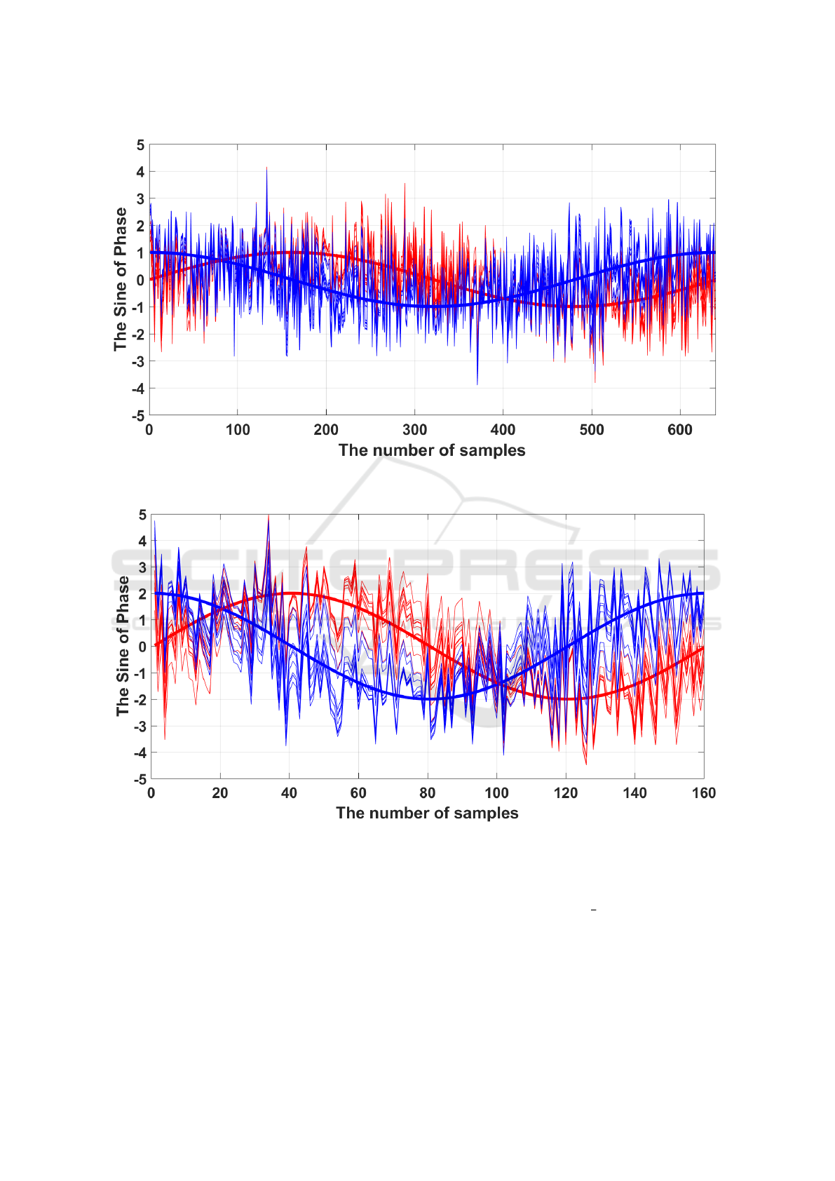
Figure 2: Ten Sinusoid signals with phase and amplitude noise compared with non-noisy signals (solid lines). Blue signals
has phase of 90 and red signals has phase of 0 degrees.
Figure 3: Ten extracted signals using Haar wavelet transform, level 2 (Approximation part). Blue signals has phase of 90 and
red signals has phase of 0 degrees.
the wave (all 64 values) and neighbouring informa-
tion from waves before and after the wave being clas-
sified. A selection of different transformations were
tried, from none at all (original signal) to Haar level
1 and 2 and db4 level 2 wavelets. Regarding using
the neighbouring information, we focused on using 7
central samples from 7 adjacent symbols (from the
target symbol and three symbols either sides). We
have found that using 7 central samples from 7 neigh-
bouring symbols gave the best linear SVM results
when we have used neighbouring information previ-
ously. In this experiment,
2
3
of the symbols/signals
were used to train the linear SVM model, and the rest
of the data (a third of the symbols) was used as a test
set.
Table 3 shows the linear SVM results using the
optical signals at the distance 8,000 km, with and
without using wavelet transform. These results were
ICPRAM 2017 - 6th International Conference on Pattern Recognition Applications and Methods
244

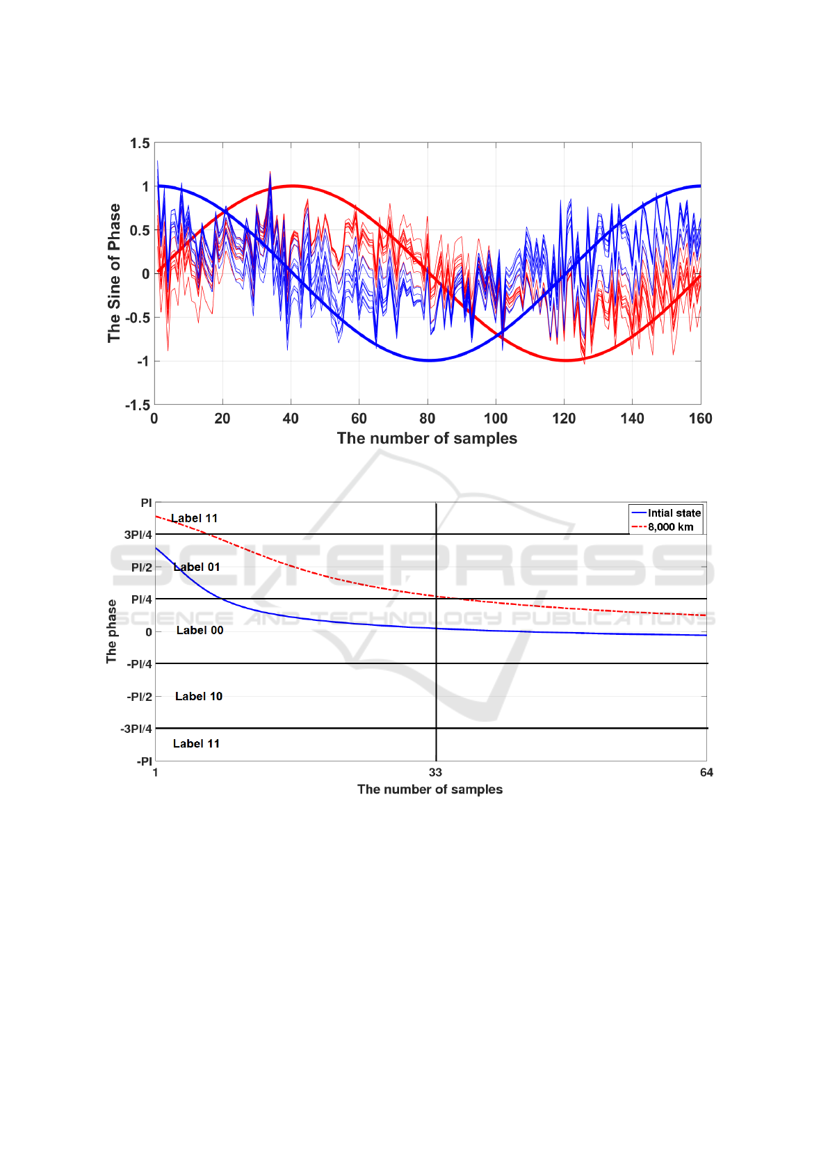
Figure 4: Ten extracted normalized signals using Haar wavelet transform, level 2 (Approximation part). Blue signals has
phase of 90 and red signals has phase of 0 degrees.
Figure 5: An optical signal has been classified incorrectly using both linear SVM using central samples from 7 symbols, Haar
transforms at level 2, and the threshold method (the first data set).
compared with the results obtained by measuring
the phase of the mid-point of the signal (threshold
method) which is the current hardware implemented
method. The Table presents the symbol accuracy rate
(SAR%), number of bit errors (NBE) and bit error rate
(BER%), which are an average over ten data sets. As
we can see from Table 3, the results using samples
from 7 consecutive symbols (using 3 either side of
the target symbol) were best, even though they only
used the central value of each of the 7 waves. This
is the result we have obtained before. Using a lin-
ear SVM using the extracted signals obtained from
DB4 wavelet transform did not improve the classifi-
cation process. The best result we have got so far is
the linear SVM result using 7 central samples from
7 neighbouring extracted signals, obtained from Haar
wavelet transform, level 2 which is a 1.68 BER.
Figures 5, 6 and 7 show some examples of optical
signals at the initial state (blue solid line), and after
8,000 km (red dotted line). The mid-point of the sig-
Error Correction over Optical Transmission
245

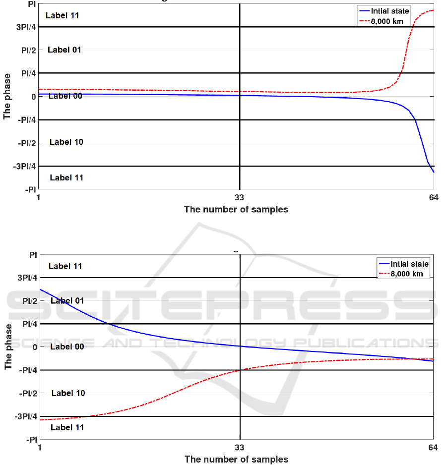
Figure 6: An optical signal has been classified correctly using both linear SVMusing central samples from 7 symbols, Haar
transforms at level 2, and the threshold method (the first data set).
Figure 7: An optical signal has been classified correctly using linear SVM using central samples from 7 symbols, Haar
transforms at level 2, and misclassified using the threshold method (the first data set).
nal is the 33
rd
sample, where the phase is measured,
because that represents the highest power level. These
figures were selected from the best linear result using
the Haar wavelet at level 2, from the target signal and
three signals either side. From Figure 5, we can see
an optical signal that has been mis-classified as class
01, using both linear SVM and the threshold method,
where it belongs to class 00. Figure 6 presents an opti-
cal signal that has been detected correctly as class 00,
using both linear SVM and the threshold method. Fig-
ure 7 shows an optical signal that has been detected
correctly using linear SVM, but incorrectly using the
threshold method. As we can see, the signal should
belong to the class 00, but was mis-classified as class
10 by the threshold method, at the distance 8,000 km.
From our observation, we can say that using linear
SVMs based on wavelets transformations can ensure
some types of distorted signals be classified correctly
(for example, Figure 7).
ICPRAM 2017 - 6th International Conference on Pattern Recognition Applications and Methods
246

Table 4: The linear SVM results using optical signals before and after using wavelet transforms at the distance 8,000 km,
compared with the threshold method result.
Method Number of samples Signal types SAR % NBE BER %
Threshold Central sample Original signal 96.3± 0.15 403.3± 16.55 1.87 ± 0.08
Linear SVM Central sample Original signal 96.29 ± 0.16 403.6 ± 18.001 1.87 ± 0.08
Linear SVM Central sample Haar level 1 96.36 ± 0.16 396.2 ± 17.37 1.84 ± 0.08
Linear SVM Central sample Haar level 2 96.41 ± 0.16 390.9 ± 17.15 1.82 ± 0.09
Linear SVM Central sample db4 level 2 93.95 ± 0.47 661.9 ± 50.71 3.07 ± 0.24
Linear SVM Whole samples Original signal 96.44 ± 0.14 387.3 ± 15.85 1.8 ± 0.07
Linear SVM Whole samples Haar level 1 96.44 ± 0.13 387.5 ± 14.22 1.8 ± 0.07
Linear SVM Whole samples Haar level 2 96.45 ± 0.13 386.2 ± 13.86 1.79 ± 0.07
Linear SVM Central samples from 7 symbols Original signal 96.6 ± 0.1 370.2 ± 11.65 1.72 ± 0.05
Linear SVM Central samples from 7 symbols Haar level 2 96.67 ± 0.11 362.4 ± 13.21 1.68 ± 0.06
Linear SVM Central samples from 7 symbols db4 level 2 95.75 ± 0.22 465.3 ± 23.45 2.16 ± 0.12
Table 2: A comparison between linear SVM results using
noisy signals and the extracted signals.
A) The whole samples of the extracted signal were used as input
to the linear SVM classifier.
Data set Type of (WT) (WT) level Accuracy rate %
P-noise
- - 92.5 %
Haar 2 91.5 %
P + A noise
- - 92.5 %
Haar 1 92.75 %
Haar 2 92.75 %
Haar 3 92.5 %
Haar 4 92.5 %
Haar 5 92.75 %
Db4 2 92.25 %
B) The central sample of the extracted signals was used as input
to the linear SVM classifier.
Data set Type of (WT) (WT) level Accuracy rate %
P-noise
- - 91.75 %
Db4 2 91.75 %
P + A noise
- - 91.75%
Haar 1 91.75%
Haar 2 91%
Haar 3 91%
Haar 4 90%
Haar 5 87.25%
Db4 2 93%
Note: P-noise means Phase noise only. P + A noise means both Phase
and Amplitude noise were used. ( - ) denotes corresponding results are
obtained without applying wavelets.
6 DISCUSSION AND
CONCLUSION
In this work, we have demonstrated that the bit error
rate can be improved by using classification based on
wavelet transforms (WT) and support vector machine
(SVM). From the results obtained using the simple
data with frequency noise in Table 1, we can see that
the best linear SVM result was when we used the
data set (AB) after using wavelet transform level 2.
Regarding the results obtained using the simple data
with phase noise in Table 2, the best linear SVM result
Table 3: A comparison between linear SVM results using
noisy signals and the extracted normalized signals.
A) The whole samples of the extracted normalized signal were
used as input to the linear SVM classifier.
Data set Type of (WT) (WT) Accuracy rate %
P-noise
- - 92.5 %
Haar 3 92.5 %
P + A noise
- - 92.5%
Haar 1 92.5%
Haar 2 92.5%
Haar 3 92.75%
Haar 4 92.5%
Haar 5 92.5%
Db4 2 92.75%
B) The central sample of the extracted normalized signal were
used as input to the linear SVM classifier.
Data set Type of (WT) (WT) Accuracy rate %
P-noise
- - 91.75 %
Db4 2 91.75 %
P + A noise
- - 91.75%
Haar 1 93.5%
Haar 2 93.5%
Haar 3 90.5%
Haar 4 93%
Haar 5 88%
Db4 2 93.75%
Note: P-noise means Phase noise only. P + A noise means both Phase
and Amplitude noise were used. ( - ) denotes corresponding results are
obtained without applying wavelets.
was when we used the central sample of the extracted
normalized signals resulted from DB4 wavelet trans-
form at level 2, which was 93.75%. Wavelets were
more beneficial with the frequency distorted data than
with the phase distorted data. However, overall the
use of wavelet transforms was disappointing.
The second part of the results were obtained using
wavelets on the optical signals at a distance of 8,000
km. The best result was when using a linear SVM
trained on the extracted data (using Haar wavelet level
2) from the target symbol and three symbols either
side. So wavelet transforms did have a small effect
on the accuracy, and in this work small effects can be
worth a lot. In particular using the combination of
Error Correction over Optical Transmission
247

neighbourhood information and wavelets gave much
better results than using the threshold method, see Ta-
ble 3. This is crucial since Bit Error Rates less than
2 are required for optical data and the further we can
drive this rate down the better. Furthermore, this work
shows that wavelet transforms can help a little with
the noise on both frequency and phase since optical
data has both.
In this paper, our initial work on wavelets has been
presented; different types of the wavelets will be in-
vestigated in the future.
REFERENCES
Bernstein, G., Rajagopalan, B., and Saha, D. (2003). Opti-
cal network control: architecture, protocols, and stan-
dards. Addison-Wesley Longman Publishing Co., Inc.
Binjumah, W., Redyuk, A., Davey, N., Adams, R., and Sun,
Y. (2015). Reducing bit error rate of optical data trans-
mission with neighboring symbol information using
a linear support vector machine. In Proceedings of
the ECMLPKDD 2015 Doctoral Consortium(2015),
pages 67–74. Aalto University.
Kanprachar, S. (1999). Modeling and analysis of the effects
of impairments in fiber optic links.
Lee, S.-H. and Lim, J. S. (2012). Parkinson’s disease clas-
sification using gait characteristics and wavelet-based
feature extraction. Expert Systems with Applications,
39(8):7338–7344.
Liu, Z., Cao, H., Chen, X., He, Z., and Shen, Z. (2013).
Multi-fault classification based on wavelet svm with
pso algorithm to analyze vibration signals from rolling
element bearings. Neurocomputing, 99:399–410.
Metaxas, A., Redyuk, A., Sun, Y., Shafarenko, A., Davey,
N., and Adams, R. (2013). Linear support vector
machines for error correction in optical data trans-
mission. In International Conference on Adaptive
and Natural Computing Algorithms, pages 438–445.
Springer.
Plonka, G., Iske, A., and Tenorth, S. (2013). Optimal rep-
resentation of piecewise h
¨
older smooth bivariate func-
tions by the easy path wavelet transform. Journal of
Approximation Theory, 176:42–67.
Rioul, O. and Vetterli, M. (1991). Wavelets and signal pro-
cessing. IEEE signal processing magazine, 8(LCAV-
ARTICLE-1991-005):14–38.
Smola, A. J. and Sch
¨
olkopf, B. (1998). Learning with ker-
nels. Citeseer.
Walker, J. S. (2008). A primer on wavelets and their scien-
tific applications. CRC press.
Wang, H., Guo, J., Wang, T., Zhang, Q., and Shao, J. (2012).
Physical layer design for free space optical commu-
nication. In Control Engineering and Communica-
tion Technology (ICCECT), 2012 International Con-
ference on, pages 978–981. IEEE.
Williams, J. R. and Amaratunga, K. (1994). Introduction to
wavelets in engineering. International Journal for Nu-
merical Methods in Engineering, 37(14):2365–2388.
ICPRAM 2017 - 6th International Conference on Pattern Recognition Applications and Methods
248